The Lyttelton port wave penetration project: Part 3

In this third mini post, I will tackle the weak formulation of the linear mild-slope equation and introduce the boundary conditions. The linear version of the equation takes into account the following physical phenomena:

Here is the equatiom:

$\nabla\cdot\left( c_p c_g \nabla \eta \right)\, +\, k^2 c_p c_g \eta = 0$

where

$\eta : \Omega(\mathbb{R} \times \mathbb{R}) \to \mathbb{C}$ is the unknown complex amplitude of the water free-surface elevation within the domain $\Omega$;
$k \in \mathbb{R}^{+}$ is the wave number;
$c_p, c_g : \Omega(\mathbb{R} \times \mathbb{R}) \to \mathbb{R}^{+}$ are respectively the phase and group velocities of the prescribed wave.

The boundary conditions will be introduced too.

I won’t discuss the derivation of the governing equation in this post.

If everything goes smoothly, at the end of that post, we should see how a monochromatic wave behaves in the Lyttelton port.

wave

Bathymetry

First thing we need to do is to gather all the data required: we already retrieved the coastline from the OSM database but we’re missing the bathymetry as both the phase speed $c_p$ and the group speed $c_g$ depend on it. Luckily Land Information New Zealand has a wonderful platform where you can access a lot of information, including nautical charts:

The second chart is a set of depth polygons and can be downloaded from LINZ as an Esri shapefile.

Then we need to lookup the depth at either each vertex or each triangle of the mesh we generated in the first part. I will consider that the depth is constant over a triangle in order to make the maths easier later on (in particular integration).

To lookup efficiently, I’m first building a spatial index of the depth polygons (I’m using a R-tree) and then query every mesh vertices. Here is how to do that in Perl:

 1 #! /usr/bin/perl
 2 use warnings;
 3 use strict;
 4 
 5 use Geo::ShapeFile;
 6 use Math::Trig 'pi';
 7 use List::Util 'min' ,'max';
 8 
 9 my $shapefile = new Geo::ShapeFile("depth-area-polygons-hydro-14k-122k");
10 $shapefile->build_spatial_index();
11 
12 my $rtree = $shapefile->get_spatial_index();
13 
14 my $d = 0.00955042966330666;
15 my $xmin = 250.816739768889;
16 my $ymin = 162.523014276134;
17 my $earthRadius = 6378137;
18 
19 my @vertices;
20 
21 open my $mesh, "< ../lyttelton.mesh";
22 while (<$mesh>) {
23 	last if /Vertices/;
24 }
25 my $nbVertex = <$mesh>;
26 foreach my $vid (1..$nbVertex) {
27 	<$mesh> =~ /^([-+]?[0-9]*\.?[0-9]+(?:[eE][-+]?[0-9]+)?)\s+([-+]?[0-9]*\.?[0-9]+(?:[eE][-+]?[0-9]+)?)\s+\d+$/;
28 
29 	my $x = $d * $1 + $xmin;
30 	my $y = $d * $2 + $ymin;
31  		
32 	# From Google mercator convertion
33     $x = 2 * pi * $earthRadius * ($x / 256 - 0.5);
34     $y = -2 * pi * $earthRadius * ($y / 256 - 0.5);
35 
36     my @shapes;
37     $rtree->query_point(($x, $y),\@shapes);
38 
39 	my $z = 12;
40 	foreach my $shape (@shapes) {
41 		if ($shape->contains_point(Geo::ShapeFile::Point->new(X => $x, Y => $y))) {
42 			my %db = $shapefile->get_dbf_record($shape->shape_id());
43 			$z = $db{'DRVAL2'};
44 			last;
45 		}
46 	}
47 	push @vertices, [$x, $y, $z];
48 }
49 
50 while (<$mesh>) {
51 	last if /Triangles/;
52 }
53 my $nbTriangle = <$mesh>;
54 foreach my $vid (1..$nbTriangle) {
55 	<$mesh> =~ /^(\d+)\s+(\d+)\s+(\d+)\s+\d+$/;
56 
57 	my $v1 = $1 - 1;
58 	my $v2 = $2 - 1;
59 	my $v3 = $3 - 1;
60 
61 	print min($vertices[$v1]->[2], $vertices[$v2]->[2], $vertices[$v3]->[2]) ."\n";
62 }

Ultimately we can display the depth (red is ~12m deep):

View Larger Map

As you can see there are some artifacts close to the border due to differences in the port geometry between the OSM and LINZ datasets. I will write a tool to fix that but it will be later.

Boundary conditions

Weak formulation

We follow the exact same steps as in the “FEM for dummies” section of the second Schur complement method post, that is, start from the governing equation, write it in the sense of distribution and apply the Green-Ostrogradsky theorem when needed. Again, I will skip all the functional analysis details regarding functional spaces. If you’re interested there is this wonderful course.

$\begin{aligned} & & \nabla\cdot\left( c_p c_g \nabla \eta \right)\, +\, k^2 c_p c_g \eta = 0\\\\ & \Leftrightarrow & \int_\Omega \psi \left\lbrace \nabla\cdot\left( c_p c_g \nabla \eta \right)\, +\, k^2 c_p c_g \eta \right\rbrace dxdy= 0, & \forall \psi \\\\ & \Leftrightarrow & \int_\Omega \psi \nabla\cdot\left( c_p c_g \nabla \eta \right)dxdy\, +\, k^2 \int_\Omega c_p c_g \psi\eta dxdy= 0\\\\ & \Leftrightarrow & \overbrace{ \int_\Omega c_p c_g \nabla \psi \nabla \eta dxdy \, +\, \oint_{\partial\Omega} c_p c_g \psi \frac{\partial \eta}{\partial n}d\sigma} \, +\, k^2 \int_\Omega c_p c_g \psi\eta dxdy= 0\end{aligned}$

Let $(e_{i})_{1 \leq i \leq N}$ a basis of the finite dimensional $\mathbb{C}$-vector space of the $\Omega(\mathbb{R} \times \mathbb{R}) \to \mathbb{C}$ piecewise linear functions over our mesh $(T_{i})_{1 \leq i \leq N}$. Let’s remark that we can choose $(e_{i})$ to be real valued tent functions so that we’re not going to compute integrals over complex valued functions.

Interior

The contribution of the first (interior) integral to the discrete operator being built is easy to compute as it has already been encountered in the second Schur complement method post.

Given $T_{i} = (q_{i_{1}},q_{i_{2}},q_{i_{3}})$, it goes:

$\begin{aligned} & & \int_{T_{i}} c_p c_g \nabla e_{i_{j}} \nabla e_{i_{k}} dxdy, & 1 \leq j,k \leq 3\\\\ & = & c_p\restriction_{T_{i}} c_g\restriction_{T_{i}} \int_{T_{i}} \nabla e_{i_{j}} \nabla e_{i_{k}} dxdy\\\\ & = & c_p\restriction_{T_{i}} c_g\restriction_{T_{i}} \frac{(q_{j^-} q_{j^+}) (q_{k^-} q_{k^+})}{4 |T_{i}|}\end{aligned}$

The contribution of the third (interior) integral goes:

$\begin{aligned} & & k^2 \int_{T_{i}} c_p c_g e_{i_{j}}e_{i_{k}} dxdy, & 1 \leq j,k \leq 3\\\\ & = & k^2 c_p\restriction_{T_{i}} c_g\restriction_{T_{i}} \int_{T_{i}} e_{i_{j}} e_{i_{k}} dxdy\\\\ & = & k^2 c_p\restriction_{T_{i}} c_g\restriction_{T_{i}} |T_{i}| \frac{(e_{i_{j}} e_{i_{k}})\bigg|_{\frac{q_{i_{1}} + q_{i_{2}}}{2}} + (e_{i_{j}} e_{i_{k}})\bigg|_{\frac{q_{i_{2}} + q_{i_{3}}}{2}} + (e_{i_{j}} e_{i_{k}})\bigg|_{\frac{q_{i_{3}} + q_{i_{1}}}{2}}}{3}\\\\ & = & \begin{cases} k^2 c_p\restriction_{T_{i}} c_g\restriction_{T_{i}} |T_{i}| \frac{0.5 * 0.5 + 0.5 * 0 + 0 * 0.5}{3} & = & k^2 c_p\restriction_{T_{i}} c_g\restriction_{T_{i}} \frac{|T_{i}|}{12} & \mbox{if } j \neq k\\\\ k^2 c_p\restriction_{T_{i}} c_g\restriction_{T_{i}} |T_{i}| \frac{0.5 * 0.5 + 0.5 * 0.5 + 0 * 0}{3} & = & k^2 c_p\restriction_{T_{i}} c_g\restriction_{T_{i}} \frac{|T_{i}|}{6} & \mbox{if } j = k\end{cases} \end{aligned}$

(We used a different 2D quadrature formula, exact for second degree polynomials.)

Border

In order to cope with the second (boundary) integral, we need to describe what’s happening near the boundary and give an expression of $\partial \eta / \partial n\restriction_{\Omega}$. Let $\Gamma_{C}$ and $\Gamma_{O}$ respectively the closed and open boundaries. Then:

$\oint_{\partial\Omega} c_p c_g \psi \frac{\partial \eta}{\partial n}d\sigma = \int_{\Gamma_{C}} c_p c_g \psi \frac{\partial \eta}{\partial n}d\sigma + \int_{\Gamma_{O}} c_p c_g \psi \frac{\partial \eta}{\partial n}d\sigma$

Closed boundary

Expression of the complex amplitude normal derivative along the closed boundary

Close to $\Gamma_{C}$, we decompose the unknown complex amplitude $\eta$ as the sum of two complex amplitudes:

the amplitude of an unknown incident wave;
the amplitude of its reflection

Here is a sketch of what’s happening:

closed boundary sketch

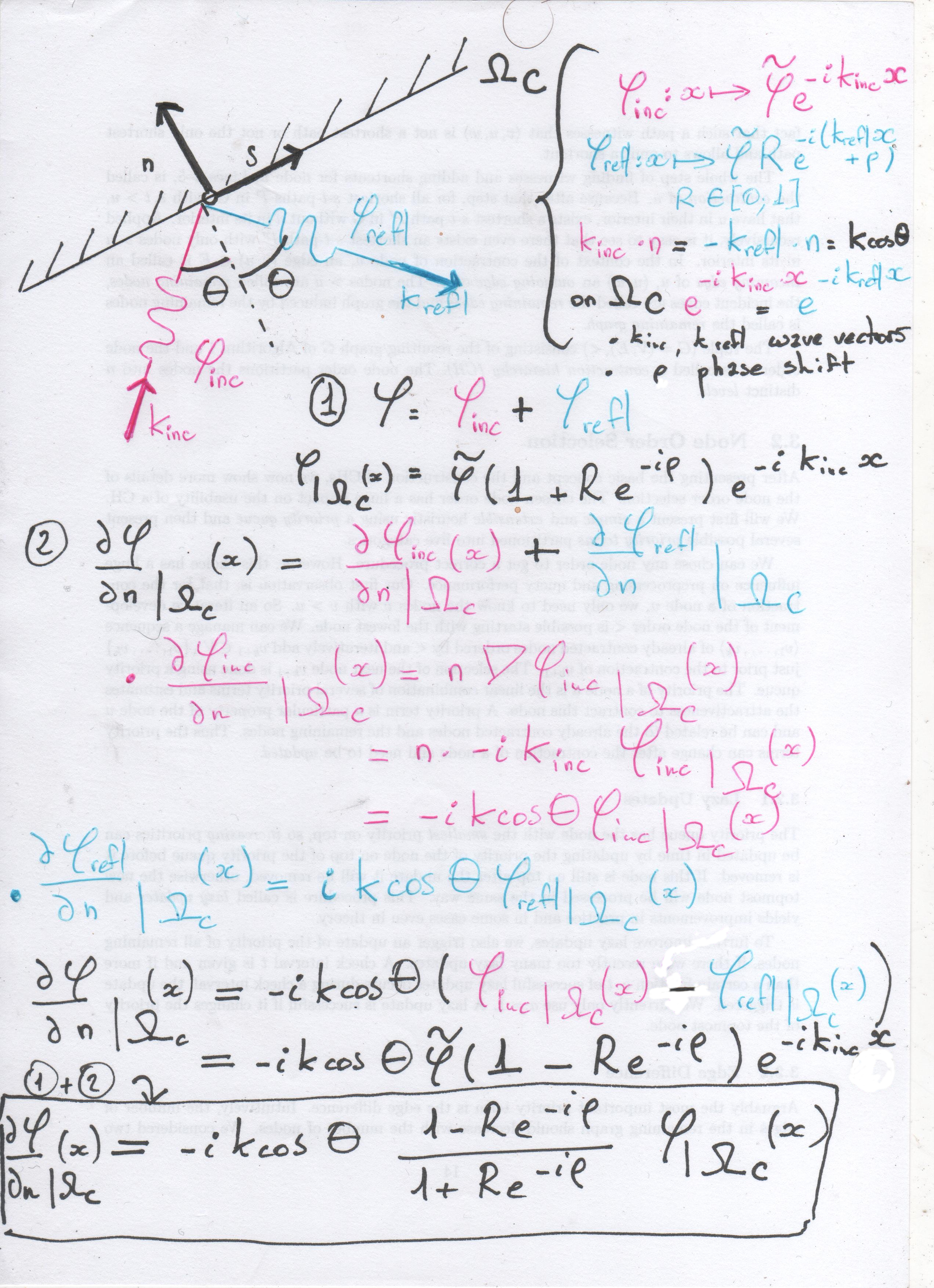
Ultimately we end up with the following expression:

$\frac{\partial \eta}{\partial n}\restriction_{\Gamma_{C}} = -i \cdot k \cdot \cos(\theta)\frac{1-Re^{-i\rho}}{1 + Re^{-i\rho}} \cdot \eta\restriction_{\Gamma_{C}}$

with $\rho$ a phase shift and $0 \leq R \leq 1$ a reflection coefficient.

We’re facing a technical difficulty as we don’t know $\theta$, the incoming wave angle. The only unknown we had so far was $\eta$, the complex amplitude of the free-surface elevation. We need to find a linear relationship between $\cos(\theta)$ and $\eta$. Here is how to find one:

Start with $\cos(\theta) = \sqrt{1 - \sin^2(\theta)}$
Use the first order Maclaurin serie of $\sqrt{1 - x}$:

$\cos(\theta) \approx 1 - \frac{\sin^2(\theta)}{2}$

Remark that

$\frac{\partial^{2} \eta}{\partial s^{2}} = \frac{\partial}{\partial s}\left(-i \cdot k \cdot \sin(\theta) \cdot \eta\right) = -k^2 \sin^2(\theta) \cdot \eta$

So that

$\cos(\theta) \approx 1 + \frac{\partial^{2} \eta / \partial s^{2}}{2 k^{2} \cdot \eta}$

and … voila:

$\frac{\partial \eta}{\partial n}\restriction_{\Gamma_{C}} \approx -i \cdot \frac{1-Re^{-i\rho}}{1 + Re^{-i\rho}} \left( k \cdot \eta + \frac{\partial^{2} \eta / \partial s^{2}}{2 k}\right)\restriction_{\Gamma_{C}}$

Since I’m implementing a baby simulator, I say that the phase shift $\rho$ is zero.

Computing the closed boundary line integral

Now that we have an expression of $\partial \eta / \partial n\restriction_{\Gamma_{C}}$ we can evaluate

$\begin{aligned} & & \int_{\Gamma_{C_{i}}} c_p c_g e_{i_{j}} \frac{\partial e_{i_{k}}}{\partial n}d\sigma, & 1 \leq j,k \leq 2\\\\ & = & -i \cdot c_p \restriction_{\Gamma_{C_{i}}} c_g \restriction_{\Gamma_{C_{i}}} \frac{1-R}{1 + R} \int_{\Gamma_{C_{i}}} e_{i_{j}} \left( k \cdot e_{i_{k}} + \frac{\partial^{2} e_{i_{k}} / \partial s^{2}}{2 k}\right)d\sigma\\\\ & = & -i \cdot c_p \restriction_{\Gamma_{C_{i}}} c_g \restriction_{\Gamma_{C_{i}}} \frac{1-R}{1 + R}\left( k \int_{\Gamma_{C_{i}}} e_{i_{j}} e_{i_{k}} d\sigma + \overbrace{\frac{1}{2k} \left( \left[ e_{i_{j}} \frac{\partial e_{i_{k}}}{\partial s} \right]_{\Gamma_{C_{i}}} - \int_{\Gamma_{C_{i}}} \frac{\partial e_{i_{j}}}{\partial s} \frac{\partial e_{i_{k}}}{\partial s}d\sigma\right)} \right)\end{aligned}$

Using Simpson’s rule we get

$\begin{aligned}& & \int_{\Gamma_{C_{i}}} e_{i_{j}} e_{i_{k}} d\sigma\\\\ & = &\frac{|\Gamma_{C_{i}}|}{6}\left((e_{i_{j}} e_{i_{k}})\bigg|_{q_{i_{1}}} + 4(e_{i_{j}} e_{i_{k}})\bigg|_{\frac{q_{i_{1}} + q_{i_{2}}}{2}} + (e_{i_{j}} e_{i_{k}})\bigg|_{q_{i_{2}}}\right)\\\\ & = &\begin{cases}\frac{|\Gamma_{C_{i}}|}{6}\left(1*0 + 4*0.5*0.5 + 0*1\right) & = & \frac{|\Gamma_{C_{i}}|}{6}, & \mbox{if } j \neq k\\\\ \frac{|\Gamma_{C_{i}}|}{6}\left(1*1 + 4*0.5*0.5 + 0*0\right) & = & \frac{|\Gamma_{C_{i}}|}{3}, & \mbox{if } j = k\\\\ \end{cases}\end{aligned}$

Remembering that $\nabla e_{i_{j} }, 1 \leq j \leq 2$ is constant along $\Gamma_{C_{i}}$

$\frac{\partial e_{i_{j} } }{\partial s} = \frac{e_{i_{j} }(q_{i_{2} }) - e_{i_{j} }(q_{i_{1} })}{|\Gamma_{C_{i} }|} = \begin{cases} \frac{0 - 1}{|\Gamma_{C_{i}}|} = -|\Gamma_{C_{i}}|^{-1}, \mbox{if } j = 1\\\\ \frac{1 - 0}{|\Gamma_{C_{i}}|} = |\Gamma_{C_{i}}|^{-1}, \mbox{if } j = 2\\\\ \end{cases}$

So that we can calculate

$\begin{aligned}& &\int_{\Gamma_{C_{i}}} \frac{\partial e_{i_{j}}}{\partial s} \frac{\partial e_{i_{k}}}{\partial s}d\sigma\\\\ & = & \frac{\partial e_{i_{j}}}{\partial s} \frac{\partial e_{i_{k}}}{\partial s} \restriction_{\Gamma_{C_{i}}} \int_{\Gamma_{C_{i}}}d\sigma\\\\ & = & \frac{\partial e_{i_{j}}}{\partial s} \frac{\partial e_{i_{k}}}{\partial s} \restriction_{\Gamma_{C_{i}}} |\Gamma_{C_{i}}|\\\\ & = & \begin{cases}-|\Gamma_{C_{i}}|^{-1} \cdot |\Gamma_{C_{i}}|^{-1} \cdot |\Gamma_{C_{i}}| & = & - |\Gamma_{C_{i}}|^{-1}, & \mbox{if } j \neq k\\\\ |\Gamma_{C_{i}}|^{-1} \cdot |\Gamma_{C_{i}}|^{-1} \cdot |\Gamma_{C_{i}}| & = & |\Gamma_{C_{i}}|^{-1}, & \mbox{if } j = k\\\\ \end{cases}\end{aligned}$

We only get a contribution from $ \left[ e_{i_{j}} \frac{\partial e_{i_{k}}}{\partial s} \right]_{\Gamma_{C_{i}}}$ at each end of the closed boundary so that I’m going to neglect it.

Open boundary

Expression of the complex amplitude normal derivative along the open boundary

Close to $\Gamma_{O}$, we decompose the unknown complex amplitude $\eta$ as the sum of two complex amplitudes:

the amplitude $\eta_{in}$ of a wave crossing $\Gamma_{O}$ towards the shore;
the amplitude $\eta_{out}$ of a wave crossing $\Gamma_{O}$ away from the shore

Here is the sketch:

open boundary sketch

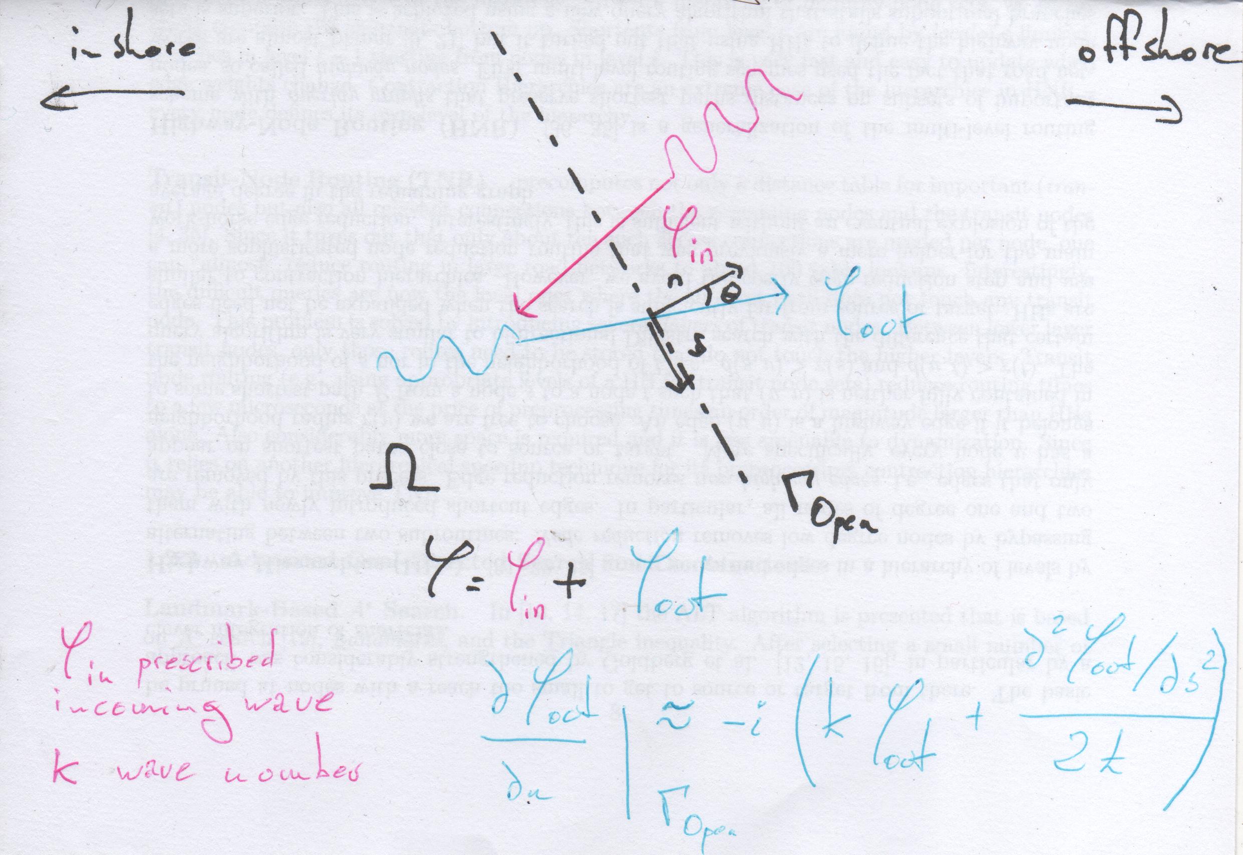
$\eta_{in}$ is given, so that computing it’s normal derivative along the open boundary is direct:

$\frac{\partial \eta_{in}}{\partial n} = -i \cdot n \cdot k_{in} \cdot \eta_{in}$

We don’t know $\theta$, the outgoing wave angle but we can reuse the approximation crafted in the previous section with $R = 0$ (no reflection) and then write back $\eta_{out}$ as the difference between $\eta$ and $\eta_{in}$:

$\begin{aligned}\frac{\partial \eta_{out}}{\partial n}\restriction_{\Gamma_{O}} & \approx & -i \cdot \left( k \cdot \eta_{out} + \frac{\partial^{2} \eta_{out} / \partial s^{2}}{2 k}\right)\restriction_{\Gamma_{O}}\\\\ & \approx & -i \cdot \left( k \cdot \left( \eta - \eta_{in} \right) + \frac{1}{2 k} \cdot \left( \frac{\partial^{2} \eta}{\partial s^{2}} - \frac{\partial^{2} \eta_{in}}{\partial s^{2}} \right)\right)\restriction_{\Gamma_{O}} \end{aligned}$

We end up with:

$\begin{aligned}\frac{\partial \eta}{\partial n}\restriction_{\Gamma_{O}} & = & -i \cdot \left( k \cdot \eta + \frac{\partial^{2} \eta / \partial s^{2}}{2 k}\right)\restriction_{\Gamma_{0}}\\\\ & + & i \cdot \left( \left(k - n \cdot k_{in}\right) \cdot \eta_{in} + \frac{\partial^{2} \eta_{in} / \partial s^{2}}{2 k}\right)\restriction_{\Gamma_{0}}\\\\ \end{aligned}$

The first term contributes to the left hand side of the linear system. The second term, involving the incoming prescribed wave, contributes to the right hand side of the linear system.

Computing the open boundary line integral

Since the first term of the normal derivative expression along the open boundary differs from the “closed” one by a $\frac{1-R}{1 + R}$ prefactor, I will only cover the computation of the second term, the contribution to the right hand side of the linear system:

$\begin{aligned} & & \int_{\Gamma_{O_{i}}} c_p c_g e_{i_{j}} \cdot i \cdot \left( \left(k - n \cdot k_{in}\right) \cdot \eta_{in} + \frac{\partial^{2} \eta_{in} / \partial s^{2}}{2 k}\right) d\sigma, & 1 \leq j\leq 2\\\\ & = & i \cdot c_p \restriction_{\Gamma_{O_{i}}} c_g \restriction_{\Gamma_{O_{i}}} \cdot \left( \left(k - n \cdot k_{in}\right) \int_{\Gamma_{O_{i}}} e_{i_{j}} \cdot \eta_{in} d\sigma + \overbrace{\frac{1}{2k} \left( \left[ e_{i_{j}} \frac{\partial \eta_{in}}{\partial s} \right]_{\Gamma_{O_{i}}} - \int_{\Gamma_{O_{i}}} \frac{\partial e_{i_{j}}}{\partial s} \frac{\partial \eta_{in}}{\partial s}d\sigma\right)}\right)\\\\ \end{aligned}$

Again, using Simpson’s rule we get

$\begin{aligned} & & \int_{\Gamma_{O_{i}}} e_{i_{j}} \cdot \eta_{in} d\sigma\\\\ & = &\frac{|\Gamma_{O_{i}}|}{6}\left((e_{i_{j}} \eta_{in})\bigg|_{q_{i_{1}}} + 4(e_{i_{j}} \eta_{in})\bigg|_{\frac{q_{i_{1}} + q_{i_{2}}}{2}} + (e_{i_{j}} \eta_{in})\bigg|_{q_{i_{2}}}\right)\\\\ & = &\begin{cases}\frac{|\Gamma_{O_{i}}|}{6}\left(1 * \eta_{in}(q_{i_{1}}) + 4*0.5*0.5*\left(\eta_{in}(q_{i_{1}}) + \eta_{in}(q_{i_{2}})\right) + 0 * \eta_{in}(q_{i_{2}})\right) & = & \frac{|\Gamma_{O_{i}}|}{6} \cdot \left( 2 * \eta_{in}(q_{i_{1}}) + \eta_{in}(q_{i_{2}}) \right), & \mbox{if } j = 1\\\\ \frac{|\Gamma_{O_{i}}|}{6}\left(0 * \eta_{in}(q_{i_{1}}) + 4*0.5*0.5*\left(\eta_{in}(q_{i_{1}}) + \eta_{in}(q_{i_{2}})\right) + 1 * \eta_{in}(q_{i_{2}})\right) & = & \frac{|\Gamma_{O_{i}}|}{6} \cdot \left( \eta_{in}(q_{i_{1}}) + 2 * \eta_{in}(q_{i_{2}}) \right), & \mbox{if } j = 2\\\\ \end{cases}\end{aligned}$

And finally,

$\begin{aligned} & & \int_{\Gamma_{O_{i}}} \frac{\partial e_{i_{j}}}{\partial s} \frac{\partial \eta_{in}}{\partial s}d\sigma\\\\ & = & \begin{cases} \int_{\Gamma_{O_{i}}} -|\Gamma_{O_{i}}|^{-1} \frac{\eta_{in}(q_{i_{2}}) - \eta_{in}(q_{i_{1}})}{|\Gamma_{O_{i}}|} d\sigma = -\frac{\eta_{in}(q_{i_{2}}) - \eta_{in}(q_{i_{1}})}{|\Gamma_{O_{i}}|}, & \mbox{if } j = 1\\\\ \int_{\Gamma_{O_{i}}} |\Gamma_{O_{i}}|^{-1} \frac{\eta_{in}(q_{i_{2}}) - \eta_{in}(q_{i_{1}})}{|\Gamma_{O_{i}}|} d\sigma = \frac{\eta_{in}(q_{i_{2}}) - \eta_{in}(q_{i_{1}})}{|\Gamma_{O_{i}}|}, & \mbox{if } j = 2\\\\ \end{cases}\end{aligned}$

Again, we neglect the $\left[ e_{i_{j}} \frac{\partial \eta_{in}}{\partial s} \right]_{\Gamma_{O_{i}}}$ term : there only is a contribution at both ends of the open boundary.

Conclusion

We’ve been through the tedious process of computing by hand all we needed to built a linear system and solve the PDE using the distributed hybrid CPU/GPU solver introduced in the previous post. Note that this time we cope with complex numbers so that the code had to be modified a little bit.

The assembly code for the mild-slope equation can be found in:

Group and phase speed, dispersion relation.

Ultimately, we will give an expression of $c_p$ the phase speed,$c_g$ the group speed as well as the product $c_p c_g$ which appears everywhere in the previously calculated expressions.

These expressions depend on the depth $h$ and we will finaly use the bathymetry information we gathered in the first part.

The Wikipedia article tells us:

The phase and group speed depend on the dispersion relation, and are derived from Airy wave theory as:
$\begin{align*} \omega^2 &=\, g\, k\, \tanh\, (kh), \\ c_p &=\, \frac{\omega}{k} \quad \text{and} \\ c_g &=\, \frac12\, c_p\, \left[ 1\, +\, kh\, \frac{1 - \tanh^2 (kh)}{\tanh\, (kh)} \right] \end{align*}$
where $g$ is Earth’s gravity and $\tanh$ is the hyperbolic tangent.

It comes

$\begin{aligned}\\\\ c_p c_g & = & \frac12 c_p^2 \left[ 1 + kh \frac{1 - \tanh^2 (kh)}{\tanh (kh)} \right]\\\\ & = & \frac{g\ \tanh (kh)}{2k} \left[ 1 + kh \frac{1 - \tanh^2 (kh)}{\tanh (kh)} \right]\\\\ \end{aligned}$

Conclusion and references

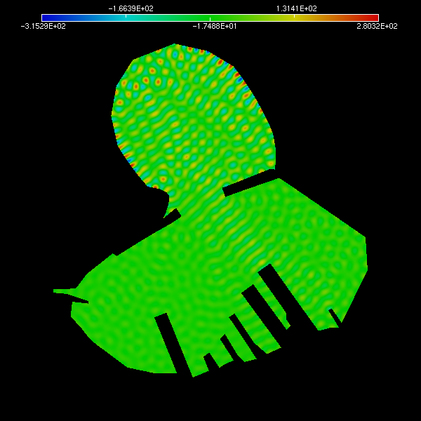
Here is the solution to the equation in the Lyttleton harbor for the following input:

3m wave length
45 degrees
harbor reflection coeff 0.9

View Larger Map

My main references were:

Wikipedia
Advanced Series on Ocean Engineering volume 13: Water Wave Propagation Over Uneven Bottoms, By Maarten W Dingemans
Acceleration of the 2D Helmholtz model HARES, By Gemma van de Sande
The Land Information New Zealand website

The next time I will modify Blender to use the solutions of my wave simulator in an attempt to render realistic coastal scenes. The workflow should be similar to the Ocean Modifier one.

← Previous Archive Next →

blog comments powered by Disqus

Published

12 April 2014