The Schur Complement Method: Part 2

We continue our informal study of domain decomposition methods (DDMs).

We will describe non-overlaping DDMs in terms of differential operators as opposed to basic linear algebra operations. This will later allow us to easily describe more sophisticated parallel algorithms such as the Dirichlet-Neuman and Neuman-Neuman algorithms.

In order to go one step further in that study it is necessary to introduce some PDE related theory and lingo. However I will try to keep it light and will just introduce what is necessary to build an intuition.

2D Poisson approximation as the Frankenstein monster

Last time we crafted an approximation, using the finite element method, of a function $\varphi$ solution of the boundary problem

$\begin{equation}\begin{cases}\Delta\varphi & = & 1, & \mbox{on } \Omega \\\ \varphi & = & 0, & \mbox{on } \partial\Omega\end{cases}\label{eq:globalPDE}\end{equation}$

Refer to the first post regarding the choice of $\Omega$ and the finite element space.

After delegating the assembly of the stiffness matrix and the load vector to the FreeFem++ software, we implemented the Schur complement method as a combination of unknown reordering and block Gaussian elimination applied to a global linear system.

In this part, I will describe how we can take into account the domain decompostion from the very begining, that is, in the formulation of the boundary problem itself.

Creating a monster

Let $\Omega_{1}$ and $\Omega_{2}$ the two non-overlaping subdomains introduced in the previous post and let $\Gamma := \partial\Omega_{1} \cap \partial\Omega_{2}$, the boundary between $\Omega_{1}$ and $\Omega_{2}$. Let $\varphi_{1}$ (respectively $\varphi_{2}$) a (local) solution of $\eqref{eq:globalPDE}$ restricted to $\Omega_{1}$ (respectively $\Omega_{2}$):

$\begin{equation}\begin{cases}\Delta\varphi_{i} & = & 1, & \mbox{on } \Omega_{i}, & i = 1,2 \\\ \varphi_{i} & = & 0, & \mbox{on } \partial\Omega_{i} \cap \partial\Omega &\end{cases}\label{eq:subdomainsPDE}\end{equation}$

Question

Is solving $\eqref{eq:subdomainsPDE}$ solving $\eqref{eq:globalPDE}$ ?

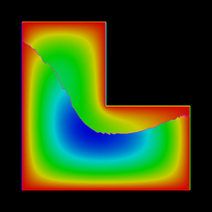
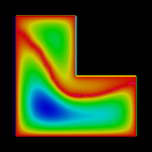
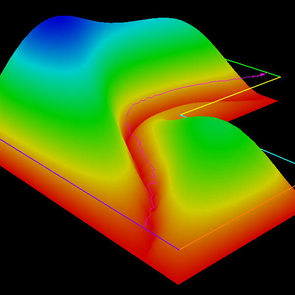
The answer is no. Here are a couple of examples to give you an intuition of what could go wrong:

Conclusion

Clearly, we need to pay more attention to what’s going on around $\Gamma$.

Trace, flux and transmission conditions

So for now, our stuff looks like this

Frankenstein

We need to add extra conditions to $\eqref{eq:subdomainsPDE}$ in order to make the global solution more regular and eventualy satisfy $\eqref{eq:globalPDE}$.

Trace

At the very least, the traces of the local solutions $\varphi_{1}$ and $\varphi_{2}$ on $\Gamma$ should be equal in order to make the global solution continous:

$\begin{equation}\varphi_{1}\restriction_\Gamma = \varphi_{2}\restriction_\Gamma\label{eq:transmissionOfTrace}\end{equation}$

Flux

Then we must ensure that the global solution is regular enough around the interface, that is, differentiable on $\Gamma$. In order to do so we will consider the normal derivatives along $\Gamma$ of the local solutions $\varphi_{1}$ and $\varphi_{2}$, also know as flux, and balance them as illustrated in the following sketch:

Flux transmission

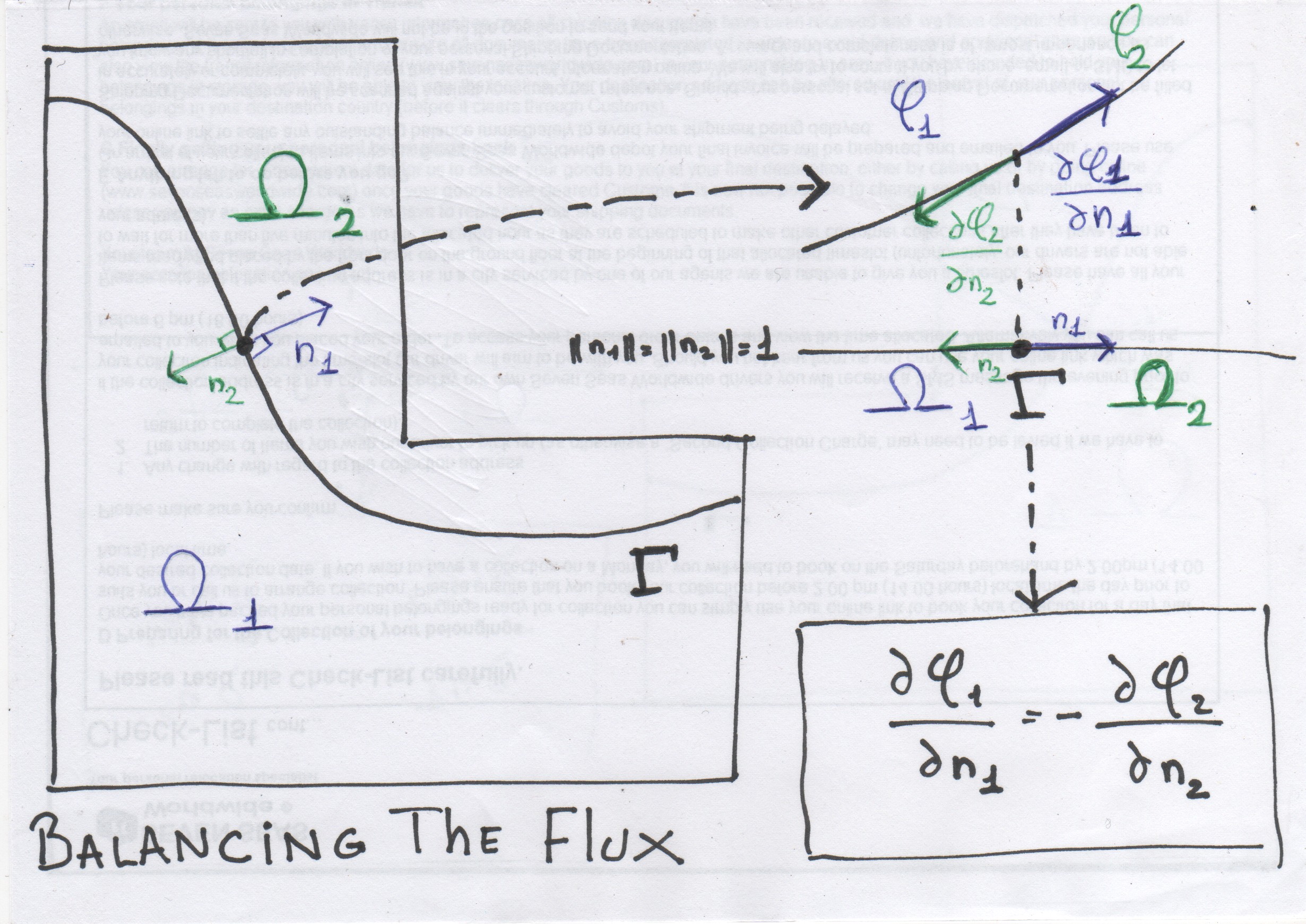
This can be concisely written as:

$\begin{equation}\frac{\partial\varphi_1}{\partial n_1} = -\frac{\partial\varphi_2}{\partial n_2}, \mbox{on } \Gamma\label{eq:transmissionOfFlux}\end{equation}$

Just remember that the directions of $n_{1}$ and $n_{2}$ depend on the point of $\Gamma$ under consideration.

$\eqref{eq:transmissionOfTrace}$ and $\eqref{eq:transmissionOfFlux}$ are known as the transmission conditions.

Putting everything together we end up with a new boundary problem:

$\begin{equation}\begin{cases}\Delta\varphi_{i} & = & 1, & \mbox{on } \Omega_{i}, & i = 1,2 \\\ \varphi_{i} & = & 0, & \mbox{on } \partial\Omega_{i} \cap \partial\Omega &\\\ \varphi_{1}\restriction_\Gamma = \varphi_{2}\restriction_\Gamma \\\ \frac{\partial\varphi_1}{\partial n_1} & = & -\frac{\partial\varphi_2}{\partial n_2}, &\mbox{on } \Gamma\end{cases}\label{eq:subdomainsPDEWithTransmition}\end{equation}$

Question

Is solving $\eqref{eq:subdomainsPDEWithTransmition}$ solving $\eqref{eq:globalPDE}$ ?

This time, under certain assumptions regarding $\Gamma$, the answer is yes but we’re not going to talk about that here.

Conclusion

We crafted a problem taking into account a 2 domains decomposition by introducing the transmission conditions: one condition related to the trace on $\Gamma$, another condition related to the flux going through $\Gamma$. Now, we’re left with a choice: either solve first for the trace or for the flux. But, before looking into that I would like to take the time to describe the main steps to translate this problem into linear algebra.

FEM for dummies

In this part I will try to explain as concisely as possible how to apply the FEM to $\eqref{eq:globalPDE}$. But please keep in mind that it is oversimplified.

Weak formulation and discretization

So far, we never discussed which functional space the solution of $\eqref{eq:globalPDE}$ should be chosen from. So let $H$ a finite-dimensional vector space of functions defined on $\Omega$ vanishing on $\partial\Omega$. Let $N:=dim(H)$ and $(e_{i})_{1 \leq i \leq N}$ a basis of $H$. I don’t want to discuss the gory functional analysis details here so just consider that I chose $H$ so that everything I’m about to write works just fine.

We will search $\varphi$ in $H$. In order to do so, we are going to design a “test” that $\varphi$ must pass in order to be a solution of $\eqref{eq:globalPDE}$. In order to design that test we choose a function $\psi$ in $H$. $\psi$ is called a test function and we say that $\varphi$ is tested against $\psi$. These are the key steps:

Weak formulation

Start with what must be satisfied: $\Delta\varphi = 1, \varphi \in H$
Multiply by a test function $\psi$: $(\Delta\varphi)\psi = \psi, \varphi \in H, \forall \psi \in H$
Sum over the domain of definition:
$\int_\Omega (\Delta\varphi)\psi dxdy = \int_\Omega \psi dxdy, \varphi \in H, \forall \psi \in H$
Apply the Green-Ostrogradsky theorem (which is a generalisation of the integration by parts we were taught back in highschool) to the sinistral side of the equation. Since $\psi$ vanishes along $\partial\Omega$, the line integral over $\partial\Omega$ vanishes too (we take into account the boundary conditions):
$\require{cancel}\begin{equation}\cancelto{0}{\oint_{\partial\Omega} \frac{\partial \varphi}{\partial n}\psi d\sigma} - \int_\Omega \nabla\varphi\nabla\psi dxdy = \int_\Omega \psi dxdy, \varphi \in H, \forall \psi \in H\label{eq:weakFormulation}\end{equation}$
Let $a: (\psi,\varphi) \mapsto \int_\Omega \nabla\psi\nabla\varphi dxdy$ and $b: \psi \mapsto -\int_\Omega \psi dxdy$. It is important to remark that $a$ (respectively $b$) is a bilinear (respectively linear) form. We can concisely re-write the previous equation:
$a(\psi,\varphi) = b(\psi), \varphi \in H, \forall \psi \in H$

Discretization

Since we chose $\psi$ in a finite-dimensional vector space, and since $a$ and $b$ are linear with respect to $\psi$. Instead of checking that the previous equation holds for any $\psi$, we just need to check that it holds for each basis vector $(e_{i})_{1 \leq i \leq N}$: $a(e_{i}, \varphi) = b(e_{i}), \varphi \in H, 1 \leq i \leq N$
Again, since we chose $\varphi$ in a finite-dimensional vector space, we can uniquely decompose $\varphi$ as a linear combination with respect to the basis $(e_{i})_{1 \leq i \leq N}$: $\varphi\ = \sum\limits_{i=1}^{N} \varphi_{i} e_{i}$. Since $a$ is linear with respect to $\varphi$, it comes:
$\sum\limits_{i=1}^{N} \varphi_{i} a(e_{i},e_{j}) = b(e_{j}), \varphi_{i} \in \mathbf{R}, 1 \leq j \leq N$
Let $A = (a(e_{i}, e_{j}))_{1 \leq i,j \leq N}$, $x = (\varphi_{i})_{1 \leq i \leq N}$ and $b = (b(e_{j}))_{1 \leq j \leq N}$. We can rewrite the previous equation as a product between a matrix and a vector :
$Ax = b, x \in \mathbf{R}^{N}$

So here we are, we started looking for $\varphi \in H$ and we end up looking for $x \in \mathbf{R}^{N}$. All we have to do now is to compute $A$ and $b$, and then solve for $x$ (note that we could just compute the effect of multiplying a vector by $A$ if we were to use an iterative solver as explained in the previous post).

Computation of the discrete operators

The next step is to compute

$\begin{aligned}A_{i,j} & = & a(e_{i}, e_{j}), 1 \leq i,j \leq N\\\ & = & \int_\Omega \nabla e_{i}\nabla e_{j} dxdy\end{aligned}$ and $\begin{aligned}b_{i} & = & b(e_{i}), 1 \leq i \leq N\\\ & = & -\int_\Omega e_{i} dxdy\end{aligned}$ but in order to do so, we must describe what are $H$ and $(e_{i})_{1 \leq i \leq N}$.

So let $H$ be the space of continuous piecewise linear functions over the triangulation of $\Omega$ (introduced in the previous post) and vanishing on $\partial \Omega$. The dimension of $H$, $N$, is equal to the number of vertices in the interior of $\Omega$.

Introducing the tent functions

So what is a basis of $H$ ? Let $(q_{i})_{1 \leq i \leq N}$ the vertices of the triangulation. Then, let’s choose $(e_{i})_{1 \leq i \leq N}$ to be the tent functions defined as follow:

$\begin{cases}e_{i} \in H\\\ e_{i}(q_{j}) = \delta_{i j}, 1\leq j \leq N \end{cases}$

and here is what a tent function looks like:

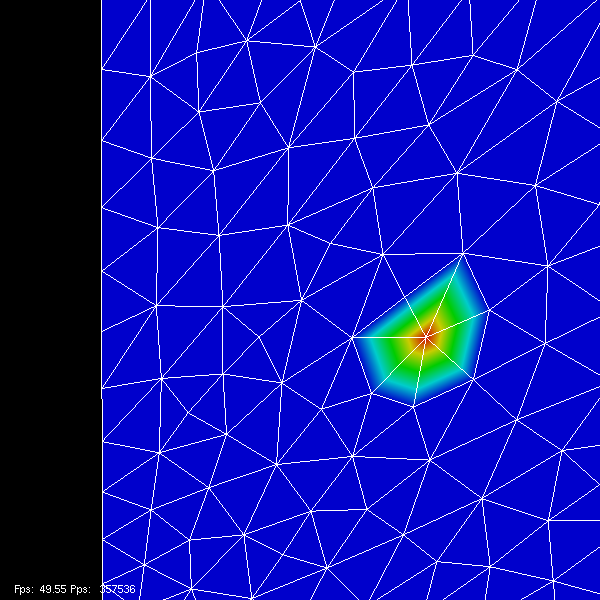
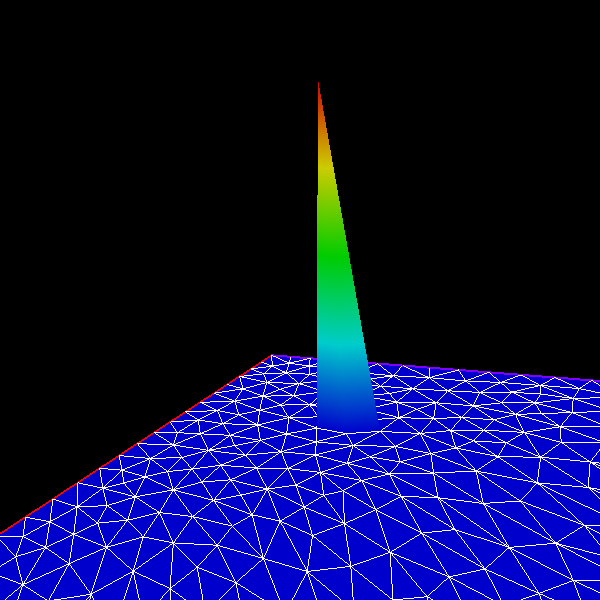
Any function in $H$ can be uniquely decompossed as a linear combination of tent functions.

We got everything we need to compute $A_{i,j}$ and $b_{i}$. We just need to walk the triangles.

Computing `$b$`

Let’s start with the easy one. Given a triangle $T_{i} = (q_{i_{1}},q_{i_{2}},q_{i_{3}})$ what are the contributions to $b$ ? We got 3 contributions: one to $b_{i_{1}}$ from $e_{i_{1}}$, one to $b_{i_{2}}$ from $e_{i_{2}}$ and one to $b_{i_{3}}$ from $e_{i_{3}}$. And the contributions are equal to:

$-\int_{T_{i}} e_{j} dxdy, j=i_{1},i_{2},i_{3}$

Now using this handy quadrature formula which is exact for affine function:

$\int_{T_{i}} f dxdy = |T_{i}|\frac{f(q_{i_{1}}) + f(q_{i_{2}}) + f(q_{i_{3}})}{3}$ where $|T_{i}|$ is the area of $T_{i}$,

If $k^- = 1 + ((k -2) \mod 3)$ and $k^+ = 1 + (k \mod 3)$, we end up with:

$\begin{aligned}-\int_{T_{i}} e_{i_{j}} dxdy & = & -|T_{i}|\frac{e_{i_{j}}(q_{i_{j^-}}) + e_{i_{j}}(q_{i_{j}}) + e_{i_{j}}(q_{i_{j^+}})}{3},& j=1,2,3\\\ & = & -|T_{i}|\frac{0 + 1 + 0}{3}\\\ & = & -\frac{|T_{i}|}{3} \end{aligned}$

Done ! Next !

Computing `$A$`

First of all, let’s remark that when $q_{i}$ and $q_{j}$ never belong to a same triangle then the supports of $e_{i}$ and $e_{j}$ are disjoint and therefore $A_{i,j}$ is zero. Otherwise, given a triangle $T_{i} = (q_{i_{1}},q_{i_{2}},q_{i_{3}})$, $e_{i_{1}}\restriction_{T_{i}}$, $e_{i_{2}}\restriction_{T_{i}}$ and $e_{i_{3}}\restriction_{T_{i}}$ being affine, their gradiants, $\nabla e_{i_{1}}\restriction_{T_{i}}$, $\nabla e_{i_{2}}\restriction_{T_{i}}$ and $\nabla e_{i_{3}}\restriction_{T_{i}}$ are constants. Therefore:

$\begin{aligned}A_{i_j,i_k} & = & \int_{T_{i}} \nabla e_{i_j}\nabla e_{i_k} dxdy , & 1 \leq j,k \leq 3\\\ & = & \nabla e_{i_j}\restriction_{T_{i}} \nabla e_{i_k}\restriction_{T_{i}} \int_{T_{i}} dxdy\\\ & = & \nabla e_{i_j}\restriction_{T_{i}} \nabla e_{i_k}\restriction_{T_{i}} |T_{i}|\end{aligned}$

So we’re left with computing $\nabla e_{i_{j}}\restriction_{T_{i}}, 1 \leq j \leq 3$. We will do that geometricaly on a sketch: Gradiant explanation

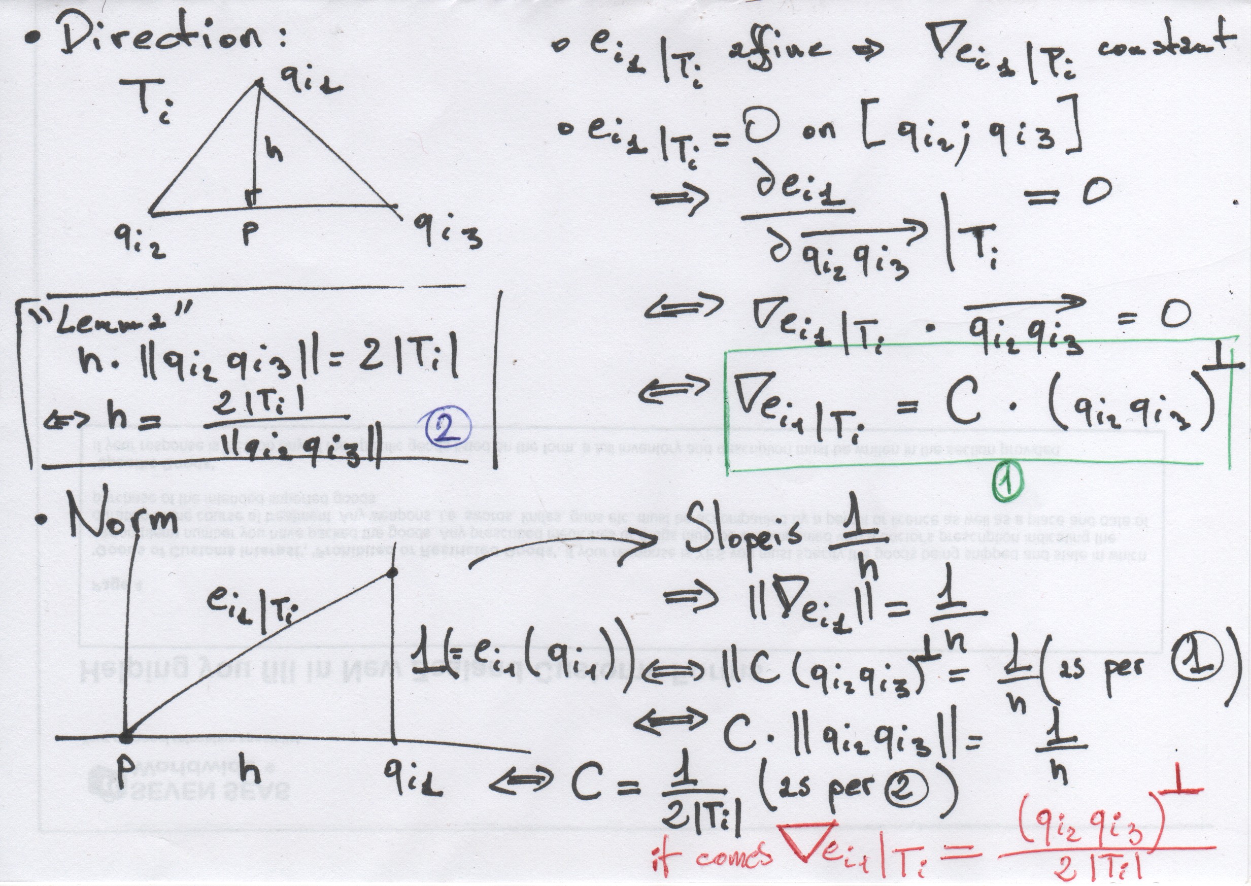
We end up with:

$\begin{aligned}A_{i_j,i_k} & = & \nabla e_{i_j}\restriction_{T_{i}} \nabla e_{i_k}\restriction_{T_{i}} |T_{i}|, & 1 \leq j,k \leq 3\\\ & = & \frac{(q_{j^-} q_{j^+})^{\perp} }{2 |T_{i}|} \frac{(q_{k^-} q_{k^+})^{\perp} }{2 |T_{i}|} |T_{i}|\\\ & = & \frac{(q_{j^-} q_{j^+}) (q_{k^-} q_{k^+})}{4 |T_{i}|}\end{aligned}$ which is easy to compute.

Implementation

We got everything now. Here is a baby implementation of the method in Javascript/WebGL.

Sub-assembling

If we apply the same procedure, restricted to each subdomain and if we use the same unknown reordering techniques introduced in the previous post, we can assemble two linear (sub-)systems:

$\left[\begin{matrix} A^{(i)}_{II} & A^{(i)}_{I\Gamma} \\\ A^{(i)}_{\Gamma I} & A^{(i)}_{\Gamma\Gamma} \end{matrix}\right]\left[\begin{matrix} x^{(i)}_{I} \\\ x^{(i)}_{\Gamma} \end{matrix}\right] = \left[\begin{matrix} b^{(i)}_{I} \\\ b^{(i)}_{\Gamma} \end{matrix}\right], i=1,2$ where

$A^{(i)}_{II}$ is the block coupling the interior of domain $i$ to itself;
$A^{(i)}_{\Gamma\Gamma}$ is the block coupling the interface to itself BUT only considering the triangles of domain $i$;
$A^{(i)}_{\Gamma I}$ is the block coupling the interface to the interior of domain $i$;
$A^{(i)}_{I\Gamma}$ is the block coupling the interior of domain $i$ to the interface

Now, given these two linear systems, we can try to write a discrete analog of $\eqref{eq:subdomainsPDEWithTransmition}$.

A discrete analog of $\eqref{eq:subdomainsPDE}$ is:

$A^{(i)}_{II} x^{(i)}_{I} + A^{(i)}_{I\Gamma} x^{(i)}_{\Gamma} = b^{(i)}_{I}, i=1,2$

But we know that is not enough, we need to take care of the transmission conditions as well.

Discrete transmition conditions

Trace

Transmission of the trace, $\eqref{eq:transmissionOfTrace}$, is simply written as:

$x^{(1)}_{\Gamma} = x^{(2)}_{\Gamma}$

Flux

Transmission of the flux, $\eqref{eq:transmissionOfFlux}$, is trickier.

How do we evaluate $\frac{\partial\varphi_i}{\partial n_i}, i=1,2$ ?

In order to do so we have to step back a little bit and re-write $\eqref{eq:weakFormulation}$ for a subdomain:

$\require{cancel}\begin{equation}\begin{aligned} & & \oint_{\partial\Omega_i} \frac{\partial \varphi_i}{\partial n}\psi d\sigma - \int_{\Omega_i} \nabla\varphi_i\nabla\psi dxdy = \int_{\Omega_i} \psi dxdy, \varphi_i \in H_i, \forall \psi \in H_i, & i=1,2\\\ & \Leftrightarrow & \cancelto{0}{\oint_{\partial\Omega_i \setminus \Gamma } \frac{\partial \varphi_i}{\partial n}\psi d\sigma} + \oint_{\Gamma } \frac{\partial \varphi_i}{\partial n_i}\psi d\sigma - \int_{\Omega_i} \nabla\varphi_i\nabla\psi dxdy = \int_{\Omega_i} \psi dxdy&\\\ & \Leftrightarrow & \oint_{\Gamma } \frac{\partial \varphi_i}{\partial n_i}\psi d\sigma = \int_{\Omega_i} \nabla\varphi_i\nabla\psi dxdy + \int_{\Omega_i} \psi dxdy& \end{aligned}\label{eq:weakNeuman}\end{equation}$

So what we have is an expression of $ \psi \mapsto \oint_{\Gamma } \frac{\partial \varphi_i}{\partial n_i}\psi d\sigma $ the dual of $\frac{\partial\varphi_i}{\partial n_i}$ in the weak topology of $H_i$. Since I said we will skip all the functional analysis details, just consider that “the flux transmission condition works the same in the weak topology”.

Particularizing $\eqref{eq:weakNeuman}$ only for $ \psi = e_{j}$ with $q_{j}$ along $\Gamma$ (otherwise the line integral is zero), a discrete analog of the “weak” flux is:

$\lambda^{(i)} := A^{(i)}_{\Gamma I} x^{(i)}_{I} + A^{(i)}_{\Gamma\Gamma} x^{(i)}_{\Gamma} - b^{(i)}_{\Gamma}$

and then the discrete analog of the “weak” flux trasmition condition is:

$\lambda^{(1)} = -\lambda^{(2)}$

Putting everything together we end up with the discrete analog of $\eqref{eq:subdomainsPDEWithTransmition}$:

$\begin{equation}\begin{cases}A^{(i)}_{II} x^{(i)}_{I} + A^{(i)}_{I\Gamma} x^{(i)}_{\Gamma} = b^{(i)}_{I}, & i=1,2\\\ x^{(1)}_{\Gamma} = x^{(2)}_{\Gamma} = x_{\Gamma}&\\\ \lambda^{(1)} = -\lambda^{(2)} = \lambda &\end{cases}\label{eq:discreteSubdomainsPDEWithTransmition}\end{equation}$

Conclusion

In that part I briefly described how to apply the FEM and to express discrete analog of the transmission conditions. In the next one, we will show how solving $\eqref{eq:discreteSubdomainsPDEWithTransmition}$ for the trace first is equivalent to what was done in the previous post.

Trace first

Remember what we did last time after massaging the global linear system ?

We first solved

$\Sigma x_{\Gamma} = \tilde{b}$

where $\Sigma = A_{\Gamma\Gamma} - A^{(1)}_{\Gamma I}(A^{(1)}_{II})^{-1}A^{(1)}_{I\Gamma} - A^{(2)}_{\Gamma I}(A^{(2)}_{II})^{-1}A^{(2)}_{I\Gamma}$ and $\tilde{b} = b_{\Gamma} - A^{(1)}_{\Gamma I}(A^{(1)}_{II})^{-1}b^{(1)}_{I} - A^{(2)}_{\Gamma I}(A^{(2)}_{II})^{-1}b^{(2)}_{I}$

and then solved

$A^{(i)}_{II}x^{(i)}_{I}= b^{(i)}_{I} − A^{(i)}_{I\Gamma}x_{\Gamma} , i=1,2$

Let’s see why it’s equivalent to solve $\eqref{eq:discreteSubdomainsPDEWithTransmition}$ for the trace first.

Previous post revisited

The idea is to craft a “trace only” equation.

From the first equation in $\eqref{eq:discreteSubdomainsPDEWithTransmition}$ comes
$x^{(i)}_{I} = (A^{(i)}_{II})^{-1}(b^{(i)}_{I} − A^{(i)}_{I\Gamma}x^{(i)}_{\Gamma}) , i=1,2$
Injecting that expression of $x^{(i)}_{I}$ in the flux transmission equation (the third equation in $\eqref{eq:discreteSubdomainsPDEWithTransmition}$) leads to
$\begin{aligned} & & \lambda^{(1)} & = -\lambda^{(2)}\\\ & \Leftrightarrow & A^{(1)}_{\Gamma I} x^{(1)}_{I} + A^{(1)}_{\Gamma\Gamma} x^{(1)}_{\Gamma} - b^{(1)}_{\Gamma} & = -(A^{(2)}_{\Gamma I} x^{(2)}_{I} + A^{(2)}_{\Gamma\Gamma} x^{(2)}_{\Gamma} - b^{(2)}_{\Gamma})\\\ & \Leftrightarrow & A^{(1)}_{\Gamma I} (A^{(1)}_{II})^{-1}(b^{(1)}_{I} − A^{(1)}_{I\Gamma}x^{(1)}_{\Gamma}) + A^{(1)}_{\Gamma\Gamma} x^{(1)}_{\Gamma} - b^{(1)}_{\Gamma} & = -(A^{(2)}_{\Gamma I} (A^{(2)}_{II})^{-1}(b^{(2)}_{I} − A^{(2)}_{I\Gamma}x^{(2)}_{\Gamma}) + A^{(2)}_{\Gamma\Gamma} x^{(2)}_{\Gamma} - b^{(2)}_{\Gamma})\end{aligned}$
Because of the trace transmission equation (the second equation in $\eqref{eq:discreteSubdomainsPDEWithTransmition}$) this is equivalent to
$\begin{aligned} & & A^{(1)}_{\Gamma I} (A^{(1)}_{II})^{-1}(b^{(1)}_{I} − A^{(1)}_{I\Gamma}x_{\Gamma}) + A^{(1)}_{\Gamma\Gamma} x_{\Gamma} - b^{(1)}_{\Gamma} & = -(A^{(2)}_{\Gamma I} (A^{(2)}_{II})^{-1}(b^{(2)}_{I} − A^{(2)}_{I\Gamma}x_{\Gamma}) + A^{(2)}_{\Gamma\Gamma} x_{\Gamma} - b^{(2)}_{\Gamma})\\\ & \Leftrightarrow & (A^{(1)}_{\Gamma\Gamma} + A^{(2)}_{\Gamma\Gamma} - A^{(1)}_{\Gamma I}(A^{(1)}_{II})^{-1}A^{(1)}_{I\Gamma} - A^{(2)}_{\Gamma I}(A^{(2)}_{II})^{-1}A^{(2)}_{I\Gamma}) x_{\Gamma} & = b^{(1)}_{\Gamma} + b^{(2)}_{\Gamma} - A^{(1)}_{\Gamma I}(A^{(1)}_{II})^{-1}b^{(1)}_{I} - A^{(2)}_{\Gamma I}(A^{(2)}_{II})^{-1}b^{(2)}_{I}\\\ & \Leftrightarrow & (A_{\Gamma\Gamma} - A^{(1)}_{\Gamma I}(A^{(1)}_{II})^{-1}A^{(1)}_{I\Gamma} - A^{(2)}_{\Gamma I}(A^{(2)}_{II})^{-1}A^{(2)}_{I\Gamma}) x_{\Gamma} & = b_{\Gamma} - A^{(1)}_{\Gamma I}(A^{(1)}_{II})^{-1}b^{(1)}_{I} - A^{(2)}_{\Gamma I}(A^{(2)}_{II})^{-1}b^{(2)}_{I}\\\ & \Leftrightarrow & \Sigma x_{\Gamma} & = \tilde{b} \end{aligned}$

That’s it ! Same !

Implementation & Conclusion

See the previous post for the details :-)

Flux first

Neumann problem

This time we need to craft a “flux only” equation.

Assemble two linear systems from $\eqref{eq:weakNeuman}$, that is, taking into account the flux, as a Neumann boundary condition:
$\begin{equation}\left[\begin{matrix} A^{(i)}_{II} & A^{(i)}_{I\Gamma} \\\ A^{(i)}_{\Gamma I} & A^{(i)}_{\Gamma\Gamma} \end{matrix}\right]\left[\begin{matrix} x^{(i)}_{I} \\\ x^{(i)}_{\Gamma} \end{matrix}\right] = \left[\begin{matrix} b^{(i)}_{I} \\\ b^{(i)}_{\Gamma} + \lambda^{(i)}\end{matrix}\right], i=1,2\label{eq:discreteNeumann}\end{equation}$
Perform the same block Gaussian elimination we did in the previous post, in order to find an expression of $x^{(i)}_{\Gamma}$:
$(A^{(i)}_{\Gamma\Gamma} - A^{(i)}_{\Gamma I}(A^{(i)}_{II})^{-1}A^{(i)}_{I\Gamma}) x^{(i)}_{\Gamma} = b^{(i)}_{\Gamma} - A^{(i)}_{\Gamma I}(A^{(i)}_{II})^{-1}b^{(i)}_{I} + \lambda^{(i)}$
concisely written as
$x^{(i)}_{\Gamma} = (\Sigma^{(i)})^{-1}(\tilde{b}^{(i)} + \lambda^{(i)})$
where $\Sigma^{(i)} := A^{(i)}_{\Gamma\Gamma} - A^{(i)}_{\Gamma I}(A^{(i)}_{II})^{-1}A^{(i)}_{I\Gamma}$ and $\tilde{b}^{(i)} := b^{(i)}_{\Gamma} - A^{(i)}_{\Gamma I}(A^{(i)}_{II})^{-1}b^{(i)}_{I}$
Inject into the trace transmission condition equation:
$\begin{aligned} & & x^{(1)}_{\Gamma} & = x^{(2)}_{\Gamma}\\\ & \Leftrightarrow & (\Sigma^{(1)})^{-1}(\tilde{b}^{(1)} + \lambda^{(1)}) & = (\Sigma^{(2)})^{-1}(\tilde{b}^{(2)} + \lambda^{(2)})\end{aligned}$
Apply the flux transmission condition:
$\begin{aligned} & & (\Sigma^{(1)})^{-1}(\tilde{b}^{(1)} + \lambda) & = (\Sigma^{(2)})^{-1}(\tilde{b}^{(2)} - \lambda)\\\ & \Leftrightarrow & ((\Sigma^{(1)})^{-1} + (\Sigma^{(2)})^{-1}) \lambda & = ((\Sigma^{(2)})^{-1} \tilde{b}^{(2)} - (\Sigma^{(1)})^{-1}\tilde{b}^{(1)})\end{aligned}$
concisely written as
$\tilde{\Sigma} \lambda = \tilde{\tilde{b}}$
where $\tilde{\Sigma} := (\Sigma^{(1)})^{-1} + (\Sigma^{(2)})^{-1}$ and $\tilde{\tilde{b}} := (\Sigma^{(2)})^{-1} \tilde{b}^{(2)} - (\Sigma^{(1)})^{-1}\tilde{b}^{(1)}$

That’s it ! Here is the “flux only” equation. All we have to do now is solve for $\lambda$, inject in $\eqref{eq:discreteNeumann}$ and solve for each subdomain.

Implementation

Here is my implementation of the “flux first” method with sub-assembling:

  1 function schurComplementMethod2()
  2 
  3    [vertices, triangles, border, domains] = readMesh("poisson2D.mesh");
  4    interface = readInterface("interface2.vids");
  5 
  6    % Assemble local Dirichlet problems 
  7    % => could be done in parallel
  8    [A1, b1, vids1] = subAssemble(vertices, triangles, border, domains, interface, 1);
  9    [A2, b2, vids2] = subAssemble(vertices, triangles, border, domains, interface, 2);
 10 
 11    nbInterior1 = length(b1) - length(interface);
 12    nbInterior2 = length(b2) - length(interface);
 13 
 14    % LU-factorize the interior of the subdomains, we're going to reuse this everywhere 
 15    % => could be done in parallel
 16    [L1, U1, p1, tmp] = lu(A1(1:nbInterior1, 1:nbInterior1), 'vector');
 17    q1(tmp) = 1:length(tmp);
 18    [L2, U2, p2, tmp] = lu(A2(1:nbInterior2, 1:nbInterior2), 'vector');
 19    q2(tmp) = 1:length(tmp);
 20 
 21    % In order to solve for the flux first, we need to compute the corresponding second member
 22    % => could be done in parallel
 23    bt1 = computeBTildI(A1, b1, nbInterior1, L1, U1, p1, q1);
 24    bt2 = computeBTildI(A2, b2, nbInterior2, L2, U2, p2, q2);
 25 
 26    epsilon = 1.e-30;
 27    maxIter = 600
 28 
 29    % Each pcg contributing to the second member could be done in parallel
 30    btt = pcg(@(x) multiplyByLocalSchurComplement(A2, nbInterior2, L2, U2, p2, q2, x), ...
 31             bt2, epsilon, maxIter) ...
 32          - pcg(@(x) multiplyByLocalSchurComplement(A1, nbInterior1, L1, U1, p1, q1, x), ...
 33             bt1, epsilon, maxIter);
 34 
 35    % Solve for the flux => each nested pcg contribution could be done in parallel
 36    flux = pcg(@(x) pcg(@(y) multiplyByLocalSchurComplement(A1, nbInterior1, L1, U1, p1, q1, y), ...
 37             x, epsilon, maxIter) ...
 38          + pcg(@(y) multiplyByLocalSchurComplement(A2, nbInterior2, L2, U2, p2, q2, y), ...
 39             x, epsilon, maxIter), btt, epsilon, maxIter);
 40 
 41    % Add the computed Neumann data to the load vectors
 42    b1(nbInterior1 + 1 : end) += flux;
 43    b2(nbInterior2 + 1 : end) -= flux;
 44    % and solve the corresponding problems using a direct method
 45    % => could be done in parallel
 46    solution = zeros(length(vertices), 1);
 47    solution(vids1) = A1 \ b1;
 48    solution(vids2) = A2 \ b2;
 49 
 50    writeSolution("poisson2D.sol", solution);
 51 
 52 endfunction
 53 
 54 function [A, b, dVertexIds] = subAssemble(vertices, triangles, border, domains, interface, domainIdx)
 55    % Keep the triangles belonging to the subdomain
 56    dTriangles = triangles(find(domains == domainIdx),:);
 57    dVertexIds = unique(dTriangles(:));
 58 
 59    % Put the interface unknowns at the end, using the numbering we computed in the last post
 60    dVertexIds = [setdiff(dVertexIds, interface); interface];
 61 
 62    % Switch domain triangles to local vertices numbering
 63    % Should use a hashtable here but their is none in octave ...
 64    globalToLocal = zeros(length(vertices), 1);
 65    globalToLocal(dVertexIds) = 1:length(dVertexIds);
 66    dTriangles(:) = globalToLocal(dTriangles(:));
 67 
 68    % Assemble the Dirichlet problem
 69    [A, b] = assemble(vertices(dVertexIds, :), dTriangles, border(dVertexIds));
 70 endfunction
 71 
 72 function [A, b] = assemble(vertices, triangles, border)
 73    nvertices = length(vertices);
 74    ntriangles = length(triangles);
 75 
 76    iis = [];
 77    jjs = [];
 78    vs = [];
 79 
 80    b = zeros(nvertices, 1);
 81    for tid=1:ntriangles
 82       q = zeros(3,2);
 83       q(1,:) = vertices(triangles(tid, 1), :) - vertices(triangles(tid, 2), :);
 84       q(2,:) = vertices(triangles(tid, 2), :) - vertices(triangles(tid, 3), :);
 85       q(3,:) = vertices(triangles(tid, 3), :) - vertices(triangles(tid, 1), :);
 86       area = 0.5 * det(q([1,2], :));
 87       for i=1:3
 88          ii = triangles(tid,i);
 89          if !border(ii)
 90             for j=1:3
 91                jj = triangles(tid,j);
 92                if !border(jj)
 93                   hi = q(mod(i, 3) + 1, :);
 94                   hj = q(mod(j, 3) + 1, :);
 95                   
 96                   v = (hi * hj') / (4 * area);
 97 
 98                   iis = [iis ii];
 99                   jjs = [jjs jj];
100                   vs = [vs v];
101                end
102             end
103             b(ii) += -area / 3;
104          end
105       end
106    end
107    A = sparse(iis, jjs, vs, nvertices, nvertices, "sum");
108 endfunction
109 
110 function [bti] = computeBTildI(A, b, nbInterior, L, U, p, q)
111    bti = b(nbInterior + 1 : end) ...
112       - A(nbInterior + 1 : end, 1:nbInterior) * (U \ (L \ b(1:nbInterior)(p)))(q);
113 endfunction
114 
115 function [res] = multiplyByLocalSchurComplement(A, nbInterior, L, U, p, q, x)
116    res = A(nbInterior + 1 : end, nbInterior + 1 : end) * x ...
117       - A(nbInterior + 1 : end, 1:nbInterior) * (U \ (L \ (A(1:nbInterior, nbInterior + 1 : end) * x)(p)))(q);
118 endfunction
119 
120 function [vertices, triangles, border, domains] = readMesh(fileName)
121 
122    fid = fopen (fileName, "r");
123 
124    % Vertices
125    fgoto(fid, "Vertices");
126    
127    [nvertices] = fscanf(fid, "%d", "C");
128    vertices = zeros(nvertices, 2);
129    for vid=1:nvertices
130       [vertices(vid, 1), vertices(vid, 2)] = fscanf(fid, "%f %f %d\n", "C");
131    end
132 
133    % Edges
134    border = zeros(nvertices, 1);
135    fgoto(fid, "Edges");
136    [nedges] = fscanf(fid, "%d", "C");
137    for eid=1:nedges
138       [v1, v2] = fscanf(fid, "%d %d %d\n", "C");
139       border(v1) = 1;
140       border(v2) = 1;
141    end
142 
143    % Elements
144    fgoto(fid, "Triangles");
145    [ntriangles] = fscanf(fid, "%d", "C");
146    triangles = zeros(ntriangles, 3);
147    domains = zeros(ntriangles, 1);
148    for tid=1:ntriangles
149       [triangles(tid, 1), triangles(tid, 2), triangles(tid, 3), domains(tid)] = fscanf(fid, "%d %d %d %d\n", "C");
150    end
151 
152    fclose(fid);
153 endfunction
154 
155 function [interface] = readInterface(fileName)
156    fid = fopen (fileName, "r");
157    interface = [];
158    while (l = fgetl(fid)) != -1
159       [vid] = sscanf(l, "%d\n", "C");
160       interface = [interface; vid];
161    end
162    fclose(fid);
163 end
164 
165 function [] = fgoto(fid, tag)
166    while !strcmp(fgetl(fid),tag)
167    end
168 endfunction
169 
170 function [] = writeSolution(fileName, solution)
171    fid = fopen (fileName, "w");
172       fprintf(fid, "MeshVersionFormatted 1\n\nDimension 2\n\nSolAtVertices\n%d\n1 1\n\n", length(solution));
173       for i=1:length(solution)
174          fprintf(fid, "%e\n", solution(i));
175       end
176       fclose(fid);
177 endfunction

Conclusion

Solving for the flux first is a bit more involved and less efficient since we have to deal with the inverse of the local Schur complement. I believe that in practice this method is never used. Nevertheless introducing the flux and the Neumann problems is a necessary step to understand the Dirichlet-Neuman and Neuman-Neuman algorithms. Someday I will try to post about that, but it will be later.

Conclusion

The next time, I would like to experiment with something more ambitious: I will try to solve the mild-slope equation in the Lyttelton port using more than two domains decompostion (trace first). I will try to use fancy stuff like MPI and GPU linear algebra libraries. Stay tuned !

View Larger Map

← Previous Archive Next →

blog comments powered by Disqus

Published

18 December 2013

The Schur Complement Method: Part 2