The Lyttelton port wave penetration project: Part 2
In this second mini-post, I’m not going to talk about the mild-slope equation : this will be for the third post. One of the main reason I’m postponing it, is that I’ve been granted access, for a limited amount of time, to a Tesla-accelerated compute cluster (kudos to Mike and Eliot). I gratefully acknowledge Microway for providing access to a Tesla-accelerated compute cluster.
The plan is to first implement a prototype of the parallel solver in Octave and then rewrite it in C++ to target the cluster.
Even though I stick to the Poisson equation, all the material presented in this post will still be usable when switching to the mild-slope equation in mini-post 3.
The Prototype
The reasons I’m spending some time writting an Octave prototype first rather than writting C++ targetting the cluster straightaway are:
- It’s easy to quickly test & debug new ideas in Octave.
- C++ makes you unproductive and I wouldn’t start writting C++ unless I know exactly where I’m going. In my opinion, writting C++ straightaway should be considered as a premature optimization.
So let’s see how we can write distributed Octave scripts.
MPI with Octave
One way of writting distributed application is via message passing. A popular message passing middleware in the HPC world is MPI.
I found two sets of Octave wrappers for MPI:
The former supports modern version of Octave (3.6-ish) but version 1.2.0 only wraps a spartan subset of the MPI API:
MPI_Comm_LoadMPI_Comm_TestMPI_Comm_rankMPI_Comm_sizeMPI_FinalizeMPI_FinalizedMPI_Get_processor_nameMPI_InitMPI_IprobeMPI_InitializedMPI_ProbeMPI_RecvMPI_Send
wheras the later wraps (almost) the entire MPI2 API but was last updated in 2007 and only support Octave 2.9.
So I decided the MPI Toolbox needed some love and spent a couple of nights making it works with modern version of Octave. It’s available on github here. I will integrate that repo in Travis CI later one. Enjoy !
We got the tool now. Let’s see how we’re going to use it.
From two to many subdomains, in parallel
I implemented a sequential two domains solver in the first two domain decomposition posts. Moving from two to many subdomains in parallel is easy enough, here is the plan:
- Each processor will assemble a local linear system involving the unknow of its subdomain plus all the interface unknows, that is, regardless of the subdomains these unknowns are interfacing. As for the two subdomains case, we distinguish between interior and interface unknowns.
- Each processor will LU-factorize the interior of its subdomain.
- Each processor will compute its contribution to the right hand side of the Schur complement system. Contributions will then be accumulated using a
MPI_Allreducecollective operation. - The processors will, collectively, solve the Schur complement system using a distributed gradient descent: every iteration of the gradient descent algorithm, each processor will compute a local contribution to the product of the Schur complement matrix with a vector. Contributions will then be accumulated using a
MPI_Allreducecollective operation. - Once the gradient descent converges, the solution for the trace is known to all the processors: they can now proceed with solving for the interior of their subdomain.
- Ultimately, a designated processor will consolidate subdomain solutions into a global solution using
MPI_Gathervcalls.
Hereafter is the Octave code doing that, including details of the gradient descent function:
 1 function mpiSchur()
 2
 3   pkg load mpitb;
 4
 5   MPI_Init;
 6
 7   [mpistatus, mpirank] = MPI_Comm_rank(MPI_COMM_WORLD);
 8   [mpistatus, mpicommsize] = MPI_Comm_size(MPI_COMM_WORLD);
 9
10   [vertices, triangles, border, interface, vids] = ...
11         readMesh("lyttelton.mesh", "interface2.vids", mpirank + 1);
12
13   % Assemble *local* stiffness matrix and load vector
14   [A, b] = assemble(vertices, triangles, border);
15
16   nbInterior = length(b) - length(interface);
17
18   % LU-factorize the interior of the subdomains, we're going to reuse this everywhere
19   [L, U, p, tmp] = lu(A(1:nbInterior, 1:nbInterior), 'vector');
20   q(tmp) = 1:length(tmp);
21
22   % We solve for the trace first: we need to compute the second member of the Schur
23   % complement system local contribution
24   bti = computeBTildI(A, b, nbInterior, L, U, p, q);
25   bt = zeros(size(bti));
26
27   % Sum contributions
28   mpistatus = MPI_Allreduce(bti, bt, MPI_SUM, MPI_COMM_WORLD);
29
30   epsilon = 1.e-30;
31   maxIter = 600;
32
33   % Solve for the trace doing distributed gradient descent
34   trcSol = pcg( @(x) parallelMultiplyBySchurComplement(A, nbInterior, L, U, p, q, x), ...
35           bt, epsilon, maxIter);
36
37   % Solve for the local interior
38   localISol = (U \ (L \ (b(1:nbInterior) - A(1:nbInterior, nbInterior + 1 : end) * trcSol)(p)))(q);
39
40   % Consolidate solutions
41   % Gather sizes of the subdomains
42   allNbInterior = zeros(mpicommsize, 1);
43   MPI_Gather(nbInterior, allNbInterior, 0, MPI_COMM_WORLD);
44
45   sumNbInterior = sum(allNbInterior);
46
47   disps = cumsum([0; allNbInterior(1:end-1)]);
48
49   % Concatenate local => global mappings of the unknowns
50   globalISol = zeros(sumNbInterior, 1);
51   MPI_Gatherv(localISol, globalISol, allNbInterior, disps, 0 , MPI_COMM_WORLD);
52
53   % Concatenate solutions
54   allVids = zeros(sumNbInterior, 1);
55   vids = vids(1:nbInterior);
56   MPI_Gatherv(vids, allVids, allNbInterior, disps, 0, MPI_COMM_WORLD);
57
58   if mpirank == 0
59     % Reorder the global solution
60     solution = zeros(sumNbInterior + length(interface), 1);
61     solution(allVids) = globalISol;
62     solution(interface) = trcSol;
63     writeSolution("lyttelton.sol", solution);
64   end
65
66   MPI_Finalize;
67 endfunction
68
69 function [res] = parallelMultiplyBySchurComplement(A, nbInterior, L, U, p, q, x)
70   % Compute the product of the *local* Schur complement with a x
71   local = A(nbInterior + 1 : end, nbInterior + 1 : end) * x ...
72     - A(nbInterior + 1 : end, 1:nbInterior) * ...
73     (U \ (L \ (A(1:nbInterior, nbInterior + 1 : end) * x)(p)))(q);
74   res = zeros(size(local));
75
76   % Sum contributions
77   MPI_Allreduce(local, res, MPI_SUM, MPI_COMM_WORLD);
78 endfunction
The entire script can be found here
Running an Octave/MPI script
I think it’s worth spending a few lines describing how to run the script as it is tricky. I’m using the Open MPI implementation of the standard.
Here is how to run an Octave/MPI script on five processors:
LD_PRELOAD=/usr/lib/libmpi.so mpirun -c 5 --tag-output octave -q --eval "mpiSchur"The LD_PRELOAD=/usr/lib/libmpi.so mpirun is necessary with Octave scripts otherwise you get an
symbol lookup error: /usr/lib/openmpi/lib/openmpi/mca_paffinity_linux.so: undefined symbol: mca_base_param_reg_intMy understanding is that the executable calling MPI_Init is expected to be linked to libmpi.so in order to work. But the octave interpreter itself is
“MPI agnostic”:
ldd $(which octave) | grep mpireturns nothing.
What, however, has been linked to libmpi.so is the set of Octave <=> C++ MPI wrappers:
ldd /usr/share/octave/packages/mpitb/MPI_Init.oct  | grep mpi
  libmpi.so.0 => /usr/lib/libmpi.so.0 (0x00007f7cda752000)
These .oct dynamic shared objects are loaded just-in-time at runtime by the interpreter, as the script consumes the MPI API, by invoking dlopen(3).
According to the man page, dlopen takes care of loading dependencies such as libmpi.so but this doesn’t seem to help.
I don’t know why but I theorize it has to do with the flags Octave pass to dlopen when loading .oct files (RTLD_LAZY vs RTLD_NOW) as well as the way the Open MPI Modular Component Architecure look-up the MPI modules.
Anyway, the workaround is to pre-load /usr/lib/libmpi.so. If you know the reason why it’s not working without pre-loading, please let me know.
Results
Here I’m sequentially displaying what is being computed in parallel:
Vectorizing assembly
In that part, I’m going to spend some time optimizing the linear system assemby.
Sloooooow …
Here is one processor performance profile as generated by the profile and profshow functions:
#                                   Function Attr     Time (s)        Calls
------------------------------------------------------------------------------
  44                          mpiSchur>assemble           199.813            1
   2                          mpiSchur>readMesh             2.664            1
  12                                     fscanf             2.199        96114
  45                                        det             0.966        17350
  47                                        mod             0.711       306330
   9                             mpiSchur>fgoto             0.681            2
  74                     mpiSchur>writeSolution             0.653            1
  69                                    fprintf             0.632        44443
  11                                   prefix !             0.512       252244
  53                                   binary \             0.434          474
   5                                      fgetl             0.371        46538
   1                                   binary +             0.328       307512
  42                        mpiSchur>fskipLines             0.287         8868
  40                                      fgets             0.279        35567
  49                                   prefix -             0.180        51361
  61 mpiSchur>parallelMultiplyBySchurComplement             0.167          235
  46                                   binary *             0.161       172159
  48                                   binary /             0.160       204995
  51                                         lu             0.117            1
  41                                      zeros             0.109        17595
It’s spending most of the time assembling the linear system.
The initial version of the assemble function loops over the triangles and then the vertices,
ignoring the border since we got a vanishing Dirichlet boundary condition.
Here is the code doing that:
 1 function [A, b] = assemble(vertices, triangles, border)
 2   nvertices = length(vertices);
 3   ntriangles = length(triangles);
 4
 5   iis = [];
 6   jjs = [];
 7   vs = [];
 8
 9   b = zeros(nvertices, 1);
10   for tid=1:ntriangles
11     q = zeros(3,2);
12     q(1,:) = vertices(triangles(tid, 1), :) - vertices(triangles(tid, 2), :);
13     q(2,:) = vertices(triangles(tid, 2), :) - vertices(triangles(tid, 3), :);
14     q(3,:) = vertices(triangles(tid, 3), :) - vertices(triangles(tid, 1), :);
15     area = 0.5 * det(q([1,2], :));
16     for i=1:3
17       ii = triangles(tid,i);
18       if !border(ii)
19         for j=1:3
20           jj = triangles(tid,j);
21           if !border(jj)
22             hi = q(mod(i, 3) + 1, :);
23             hj = q(mod(j, 3) + 1, :);
24
25             v = (hi * hj') / (4 * area);
26
27             iis = [iis ii];
28             jjs = [jjs jj];
29             vs = [vs v];
30           end
31         end
32         b(ii) += -area / 3;
33       end
34     end
35   end
36   A = sparse(iis, jjs, vs, nvertices, nvertices, "sum");
37 endfunction
An efficient way to perform the assembly of finite element matrices in Matlab and Octave
Some people say Octave sucks at loops. Suffice it to say it’s much better at vector operations as we will see. I made a few research about vectorizing FEM linear system assembly and found an awesome May 2013 research report by François Cuvelier, Caroline Japhet & Gilles Scarella at Inria titled “An efficient way to perform the assembly of finite element matrices in Matlab and Octave” Exactly what I needed. Hereafter is the new version applying technics from these guys research:
 1 function [A, b] = assemble(vertices, triangles, border)
 2   nvertices = length(vertices);
 3   ntriangles = length(triangles);
 4
 5   q1 = vertices(triangles(:, 1), :);
 6   q2 = vertices(triangles(:, 2), :);
 7   q3 = vertices(triangles(:, 3), :);
 8
 9   u = q2 - q3;
10   v = q3 - q1;
11   w = q1 - q2;
12
13   a(:,1,:) = v';
14   a(:,2,:) = w';
15   areas = 0.5 * cellfun(@det, num2cell(a,[1,2]))(:);
16   areas4 = 4 * areas;
17
18   val(:, 1) = sum(u.*u, 2) ./ areas4;
19   val(:, 2) = sum(u.*v, 2) ./ areas4;
20   val(:, 3) = sum(u.*w, 2) ./ areas4;
21   val(:, 5) = sum(v.*v, 2) ./ areas4;
22   val(:, 6) = sum(v.*w, 2) ./ areas4;
23   val(:, 9) = sum(w.*w, 2) ./ areas4;
24   val(:, [ 4 , 7 , 8]) = val(:, [ 2 , 3 , 6 ]);
25
26   col = triangles(:, [1 1 1 2 2 2 3 3 3]);
27   row = triangles(:, [1 2 3 1 2 3 1 2 3]);
28
29   A = sparse(col(:), row(:), val(:), nvertices, nvertices);
30   % Dirichet penalty
31   A += spdiags(1e30 * !!border, [0], nvertices, nvertices);
32
33   b = zeros(nvertices, 1);
34   for tid=1:ntriangles
35     b(triangles(tid,:)) += -areas(tid) / 3;
36   end
37
38 endfunction
Dirichlet penalty
In the vectorized assembly, I also used a trick of the trade (ripped off from FreeFem++) to handle the Dirichlet boundary condition without testing for boundary vertices:
treat these vertices as unknowns in their own rights, tweaking coefficients of the linear system
so that the solution on the boundary matches the Dirichlet condition. It’s sometime refered as “handling
Dirichlet boundary condition with a penalty”. Let’s say we want to make \(x_{i}\) equal to \(d\) in the solution. Here is how it goes:
choose a very very large value \(P\) (the penalty), add \(P * d\) to \(b_{i}\) in the load vector and add \(P\) to \(A_{i,i}\) in the stiffness matrix.
And … \(A_{i}x \thickapprox A_{i,i}x_{i} \thickapprox P*x_{i} = b_{i} \thickapprox P*d\) which is the same as \(x_{i} = d\).
… Fast
Here is the new perf profile:
#                                   Function Attr     Time (s)        Calls
------------------------------------------------------------------------------
   2                          mpiSchur>readMesh             2.900            1
  12                                     fscanf             2.453        96114
  63                                   binary \             2.366         2006
  71 mpiSchur>parallelMultiplyBySchurComplement             0.741         1001
   9                             mpiSchur>fgoto             0.703            2
  80                     mpiSchur>writeSolution             0.655            1
  81                                    fprintf             0.635        44441
  66                              MPI_Allreduce             0.479         1002
   5                                      fgetl             0.394        46538
  44                          mpiSchur>assemble             0.368            1
  42                        mpiSchur>fskipLines             0.285         8868
  40                                      fgets             0.281        35567
  67                                        pcg             0.229            1
  48                                        det             0.211        17350
  49                                   binary *             0.112         7009
  13                                  binary ==             0.086        87273
  61                                         lu             0.073            1
  70                                      feval             0.056         1001
  10                                     strcmp             0.042        46104
  11                                   prefix !             0.038        46113
0.368s instead of 199.813s, not too bad ;-)
Another good reason to spend time vectorizing Octave code is that it’s easier to make good use of the GPUs or translate the code into Cuda kernels as we will see.
Note that I didn’t take advantage of the symmetric structure of the linear system (I will do that in the C++ version of the solver) because I could not find a way to use the Sparse and matrix_type functions together to tell Octave that the matrix is symmetric allowing me to only store the upper triangular part. If you know how to do that, please tell me.
Tesla-accelerated compute cluster
In that part I will describe Microway’s Test Drive Cluster hardware as well as how to compile and run software targetting it.
Cluster hardware
I will be using the “benchmark” partition of the cluster:
[seba@head ~]$ sinfo
PARTITION   AVAIL  TIMELIMIT  NODES  STATE NODELIST
month-long   down 31-00:00:0      1  alloc node3
week-long      up 7-00:00:00      1  alloc node3
day-long       up 1-00:00:00      1  alloc node3
day-long       up 1-00:00:00      2   idle node[4-5]
day-long       up 1-00:00:00      1   down node2
benchmark*     up    8:00:00      1  alloc node3
benchmark*     up    8:00:00      2   idle node[4-5]
benchmark*     up    8:00:00      1   down node2
short          up      30:00      1  alloc node3
short          up      30:00      2   idle node[4-5]
short          up      30:00      1   down node2
interactive    up    8:00:00      1  alloc node3
interactive    up    8:00:00      2   idle node[4-5]
interactive    up    8:00:00      1   down node2
A partition is a subset of the cluster. At that time, the “benchmark” partition has 3 nodes up:
| Node | CPUs | Memory | GPUs |
|---|---|---|---|
| I node3 | I 2x 10-core Xeon E5-2680v2 @ 2.80GHz | I 64GB DDR3 1866MHz | I 2x NVIDIA Tesla K40 |
| I node4 | I 2x 10-core Xeon E5-2680v2 @ 2.80GHz | I 64GB DDR3 1866MHz | I 2x NVIDIA Tesla K40 |
| I node5 | I 2x 10-core Xeon E5-2680v2 @ 2.80GHz | I 128GB DDR3 1866MHz | I 3x NVIDIA Tesla K20 |
The nodes use InfiniBand to talk to each others:
[seba@head ~]$ ip addr show ib0
4: ib0: <BROADCAST,MULTICAST,UP,LOWER_UP> mtu 2044 qdisc pfifo_fast state UP qlen 256
    link/infiniband 80:00:00:48:fe:80:00:00:00:00:00:00:00:1e:67:03:00:29:47:6f brd 00:ff:ff:ff:ff:12:40:1b:ff:ff:00:00:00:00:00:00:ff:ff:ff:ff
    inet 10.10.0.254/16 brd 10.10.255.255 scope global ib0
    inet6 fe80::21e:6703:29:476f/64 scope link
       valid_lft forever preferred_lft forever
Cluster environment
SLURM

Cluster ressources management is handled by SLURM.
SLURM allows you to submit jobs into a priority queue.
A job priority depends on several factors among which the ressources required by the job.
SLURM provides command such as sinfo, sbatch, srun, scancel, squeue to manage jobs.
Job submission is done passing a submission script to the sbatch command.
A submission script is just a shell script with extra directives in comment.
For example here is the submission script I’m using to run babyhares with 5 processors on two nodes with 6 CPUs (cores) by processor and 2 K40 GPUs per node:
#!/bin/bash

# Describe the required ressources
#SBATCH --ntasks=5 --cpus-per-task=6 --nodes=2
#SBATCH --gres=gpu:2
#SBATCH --constraint=K40
#SBATCH --mem=32768
#SBATCH --time=10:00
#SBATCH --job-name=LytteltonWaveSimulation
#SBATCH --error=LytteltonWaveSimulation.%j.output.errors
#SBATCH --output=LytteltonWaveSimulation.%j.output.log
gpus_per_node=2
source /mcms/core/slurm/scripts/libexec/slurm.jobstart_messages.sh

# Setup the runtime environment
# Intel C++/MKL runtime
module load intel
# MPI over infiniband
module load mvapich2
# Cuda
module load cuda
module list 2>&1
echo; echo;

# Run the parallel solver (srun works like mpirun), never worked without --exclusive
# If using OpenMPI, you can use mpirun
srun -vvvvvvv -n 5 -c 6 -N 2 --exclusive /home/seba/work/ssrb.github.com/assets/lyttelton/BabyHares/babyhares_k40 /home/seba/work/ssrb.github.com/assets/lyttelton/BabyHares/lyttelton.mesh /home/seba/work/ssrb.github.com/assets/lyttelton/BabyHares/interface2.vids
Then we can submit the job and check that it’s indeed queued. Like so:
[seba@head ~]$ sbatch -v work/ssrb.github.com/assets/lyttelton/seba-babyhares-lyttelton-port-5-subdomains-TeslaK40.sh
sbatch: auth plugin for Munge (http://code.google.com/p/munge/) loaded
Submitted batch job 18
[seba@head ~]$ squeue
             JOBID PARTITION     NAME     USER ST       TIME  NODES NODELIST(REASON)
                18 benchmark Lyttelto     seba PD       0:00      2 (Resources)
                 5 week-long vlao-job     vlao  R 1-20:30:06      1 node3
As we can see in this example, a job is currently running on one of the K40 node (node3). Since I just wanted to demonstrate job submission, I will cancel my job:
[seba@head ~]$ scancel 18
[seba@head ~]$ squeue
             JOBID PARTITION     NAME     USER ST       TIME  NODES NODELIST(REASON)
                 5 week-long vlao-job     vlao  R 1-20:39:21      1 node3
Depending on SLURM’s configuration, a job can pre-empt another one based on its priority.
On the cluster, the SLURM scheduler isn’t configured to be pre-emptive:
[seba@head ~]$ sinfo -a -o  "%P %p %M"
PARTITION PRIORITY PREEMPT_MODE
month-long 5000 OFF
week-long 10000 OFF
day-long 20000 OFF
benchmark* 30000 OFF
short 40000 OFF
interactive 50000 OFF
My understandig is that my job would never have interfered with the other job even though the “benchmark” partition priority is greater than the “week-long” partition one.
I noticed that I can’t book all the 40 CPUs on the two K40 nodes for a single job. The limit seems to be 30 CPUs. My guess is that the 10 CPUs for the “interactive” partition should always be available, but I’m not sure. If you know the reason, please tell me.
Enough SLURM !

lmod
Node configuration is handled using lmod. It allows you to easily switch compilers, MPI implementations, Cuda versions and so one. Here is an example of what lmod is doing:
[seba@head ~]$ interactive -g gpu:2 -f K40
salloc: Granted job allocation 22
srun: Job step created
[seba@node3 ~]$ echo $LD_LIBRARY_PATH
/mcms/core/slurm/lib:/usr/lib64/nvidia:/usr/local/cuda-5.5/lib64
[seba@node3 ~]$ mpicc
bash: mpicc : commande introuvable ;-)
[seba@node3 ~]$ module load gcc
[seba@node3 ~]$ module load openmpi
[seba@node3 ~]$ echo $LD_LIBRARY_PATH
/mcms/core/openmpi/1.7.3/gcc/4.4.7/lib:/mcms/core/slurm/lib:/usr/lib64/nvidia:/usr/local/cuda-5.5/lib64
[seba@node3 ~]$ mpicc -show
gcc -I/mcms/core/openmpi/1.7.3/gcc/4.4.7/include -pthread -L/mcms/core/openmpi/1.7.3/gcc/4.4.7/lib -lmpi
[seba@node3 ~]$ module swap gcc intel

Due to MODULEPATH changes the following have been reloaded:
  1) openmpi/1.7.3

[seba@node3 ~]$ echo $LD_LIBRARY_PATH
/mcms/core/openmpi/1.7.3/intel/2013_sp1.0.080/lib:/opt/intel/composer_xe_2013_sp1.0.080/tbb/lib/intel64/gcc4.4:/opt/intel/composer_xe_2013_sp1.0.080/mkl/lib/intel64:/opt/intel/composer_xe_2013_sp1.0.080/ipp/lib/intel64:/opt/intel/composer_xe_2013_sp1.0.080/mpirt/lib/intel64:/opt/intel/composer_xe_2013_sp1.0.080/compiler/lib/intel64:/mcms/core/slurm/lib:/usr/lib64/nvidia:/usr/local/cuda-5.5/lib64
[seba@node3 ~]$ mpicc -show
icc -I/mcms/core/openmpi/1.7.3/intel/2013_sp1.0.080/include -pthread -L/mcms/core/openmpi/1.7.3/intel/2013_sp1.0.080/lib -lmpi
[seba@node3 ~]$ module swap openmpi mvapich2
[seba@node3 ~]$ mpicc -show
icc -I/mcms/core/slurm/2.6.5/include -I/usr/local/cuda-5.5/include -L/mcms/core/slurm/2.6.5/lib64 -L/mcms/core/slurm/2.6.5/lib -L/usr/local/cuda-5.5/lib64 -L/usr/local/cuda-5.5/lib -L/mcms/core/slurm/2.6.5/lib64 -L/mcms/core/slurm/2.6.5/lib -I/mcms/core/mvapich2/1.9/intel/2013_sp1.0.080/include -L/mcms/core/mvapich2/1.9/intel/2013_sp1.0.080/lib -Wl,-rpath -Wl,/mcms/core/mvapich2/1.9/intel/2013_sp1.0.080/lib -lmpich -lpmi -lopa -lmpl -lcudart -lcuda -libmad -lrdmacm -libumad -libverbs -lrt -lhwloc -lpmi -lpthread -lhwloc
I noticed that when loading Cuda and OpenMPI with either gcc or icc, the Cuda related compiler switches are not added by lmod:
[seba@node3 ~]$ module load gcc
[seba@node3 ~]$ module load openmpi
[seba@node3 ~]$ mpicc -show
gcc -I/mcms/core/openmpi/1.7.3/gcc/4.4.7/include -pthread -L/mcms/core/openmpi/1.7.3/gcc/4.4.7/lib -lmpi
[seba@node3 ~]$ module load cuda
[seba@node3 ~]$ mpicc -show
gcc -I/mcms/core/openmpi/1.7.3/gcc/4.4.7/include -pthread -L/mcms/core/openmpi/1.7.3/gcc/4.4.7/lib -lmpi
[seba@node3 ~]$ module swap gcc intel

Due to MODULEPATH changes the following have been reloaded:
  1) openmpi/1.7.3

[seba@node3 ~]$ mpicc -show
icc -I/mcms/core/openmpi/1.7.3/intel/2013_sp1.0.080/include -pthread -L/mcms/core/openmpi/1.7.3/intel/2013_sp1.0.080/lib -lmpi
so that if you want to compile OpenMPI+Cuda code you have to add these switches yourself:
mpicc -I/usr/local/cuda-5.5/include -L/usr/local/cuda-5.5/lib64 -L/usr/local/cuda-5.5/lib -lcuda -lcudart -lcusparseMaybe we’re supposed to always use mvapich2 ?
I also noticed that when using mvapich2, the rdmacm, ibumad, ibverbs and hwloc libraries cannot be found by mpicc so that you can’t compile out of the box.
I believe that’s because these libs are missing the “.so” symlinks in /usr/lib64. Anyway you don’t have to explicitely link
with these InfiniBand/hwloc related libs as shown by ldd:
[seba@node3 ~]$ module load intel
[seba@node3 ~]$ module load mvapich2
[seba@node3 BabyHares]$ mpicc -pthread  -openmp -mkl=parallel -lcusparse *.cpp -o babyhares
ld: cannot find -libmad
[seba@node3 BabyHares]$ mpicc -show
icc -I/mcms/core/slurm/2.6.5/include -I/usr/local/cuda-5.5/include -L/mcms/core/slurm/2.6.5/lib64 -L/mcms/core/slurm/2.6.5/lib -L/usr/local/cuda-5.5/lib64 -L/usr/local/cuda-5.5/lib -L/mcms/core/slurm/2.6.5/lib64 -L/mcms/core/slurm/2.6.5/lib -I/mcms/core/mvapich2/1.9/intel/2013_sp1.0.080/include -L/mcms/core/mvapich2/1.9/intel/2013_sp1.0.080/lib -Wl,-rpath -Wl,/mcms/core/mvapich2/1.9/intel/2013_sp1.0.080/lib -lmpich -lpmi -lopa -lmpl -lcudart -lcuda -libmad -lrdmacm -libumad -libverbs -lrt -lhwloc -lpmi -lpthread -lhwloc
# Removing -libmad -lrdmacm -libumad -libverbs -lhwloc
[seba@node3 BabyHares]$ icc -I/mcms/core/slurm/2.6.5/include -I/usr/local/cuda-5.5/include -L/mcms/core/slurm/2.6.5/lib64 -L/mcms/core/slurm/2.6.5/lib -L/usr/local/cuda-5.5/lib64 -L/usr/local/cuda-5.5/lib -I/mcms/core/mvapich2/1.9/intel/2013_sp1.0.080/include -L/mcms/core/mvapich2/1.9/intel/2013_sp1.0.080/lib -Wl,-rpath -Wl,/mcms/core/mvapich2/1.9/intel/2013_sp1.0.080/lib -lmpich -lpmi -lopa -lmpl -lcudart -lcuda -lrt -lpthread  -openmp -mkl=parallel -lcusparse  *.cpp -o babyhares
[seba@node3 BabyHares]$ echo $?
0
[seba@node3 BabyHares]$ ldd babyhares
  ...
  libmpich.so.10 => /mcms/core/mvapich2/1.9/intel/2013_sp1.0.080/lib/libmpich.so.10 (0x00007f11b7eaa000)
  ...
  libibmad.so.5 => /usr/lib64/libibmad.so.5 (0x00007f11a9c72000)
  librdmacm.so.1 => /usr/lib64/librdmacm.so.1 (0x00007f11a9a5d000)
  libibumad.so.3 => /usr/lib64/libibumad.so.3 (0x00007f11a9857000)
  libibverbs.so.1 => /usr/lib64/libibverbs.so.1 (0x00007f11a964a000)
  libslurm.so.26 => /mcms/core/slurm/2.6.5/lib/libslurm.so.26 (0x00007f11a9328000)
  libhwloc.so.5 => /usr/lib64/libhwloc.so.5 (0x00007f11a9100000)
  ...
[seba@node3 BabyHares]$ ldd /mcms/core/mvapich2/1.9/intel/2013_sp1.0.080/lib/libmpich.so.10
  ...
  libibmad.so.5 => /usr/lib64/libibmad.so.5 (0x00007f8bb3933000)
  librdmacm.so.1 => /usr/lib64/librdmacm.so.1 (0x00007f8bb371f000)
  libibumad.so.3 => /usr/lib64/libibumad.so.3 (0x00007f8bb3519000)
  libibverbs.so.1 => /usr/lib64/libibverbs.so.1 (0x00007f8bb330b000)
  ...
The C++ Solver
In that part I will discuss some of the C++ code. Since I will be using the Intel compiler, I won’t use C++11 as it’s not well supported. The code can be found here.
Hybrid CPU/GPU linear system assembly
The Octave prototype assembles a single linear system for each subdomain and then accesses the different blocks using range indexing. In C++, I will manipulate 3 matrices, the “interior-interior” matrix, the “interface-interface” matrix and the “interior-interface” matrix. The matrices will be stored in CSR format. This time we take advantage of the symmetry of the “interior-interior” and “interface-interface” matrices.
Computing the profile of the matrices is done on the CPU.
void  PartialDifferentialEquation::countNZCoefficents(const MeshConstPtr &mesh) {

int nbInteriorVertices = mesh->_vertices.size() - mesh->_nbInterfaceVertices;

_nbNonNullCoefficentsAII = 0;
_nbNonNullCoefficentsAIG = 0;
_nbNonNullCoefficentsAGG = 0;

std::vector<int> color(mesh->_vertices.size(), -1);
for (int row = 0; row < mesh->_vertices.size(); ++row) {
   const Vertex &vi(mesh->_vertices[row]);
   // Inspect each triangle connected to vertex row
   for (RCTI ti = _rct.find(row); ti != _rct.end(); ++ti) {
     const Triangle &triangle(mesh->_triangles[*ti]);
     for (int sj = 0; sj < 3; ++sj) {
       int column = triangle.v[sj];
       const Vertex &vj(mesh->_vertices[column]);
       // Do not count coefficient twice
       if (color[column] != row) {
         color[column] = row;
         // AII or AIG
         if (row < nbInteriorVertices) {
           // AII
           if (column < nbInteriorVertices) {
             // AII is symmetric
             if (row <= column) {
              ++_nbNonNullCoefficentsAII;
             }
           // AIG
           } else {
            ++_nbNonNullCoefficentsAIG;
           }
          // AGG
          } else {
            // AGG is symmetric
            if (row <= column) {
             ++_nbNonNullCoefficentsAGG;
            }
          }
        }
      }
    }
  }
}
In order to efficiently iterate over the triangles connected to a given vertex in the previous code, we need to build a reverse connectivity table:
#pragma once
#include "Mesh.h"

#include <vector>

namespace BabyHares {
  class ReverseConnectivityTable {
    public:
      void init(const MeshConstPtr &mesh) {
        _head.resize(mesh->_vertices.size(), -1);
        _next.resize(3 * mesh->_triangles.size());
        for (int ti = 0, p = 0; ti < mesh->_triangles.size(); ++ti) {
          for (int si = 0; si < 3; ++si, ++p) {
            int vi = mesh->_triangles[ti].v[si];
            _next[p] = _head[vi];
            // (p / 3) = ti, is the triangle number,
            // the new head of the list of triangles for vertex vi;
            _head[vi] = p;
          }
        }
      }

      class Iter {
        public:
          friend class ReverseConnectivityTable;
          const Iter operator++() {
            _p = _rct->_next[_p];
            return *this;
          }
          int operator*() const{
            return _p / 3;
          }
          bool operator!=(const Iter &rhs) const {
            return  _p != rhs._p || _rct != rhs._rct;
          }
        private:
          const ReverseConnectivityTable *_rct;
          int _p;
      };

      Iter find(int vi) const {
        Iter iter;
        iter._rct = this;
        iter._p = _head[vi];
        return iter;
      }

      Iter end() const {
        Iter iter;
        iter._rct = this;
        iter._p = -1;
        return iter;
      }

    private:
      std::vector<int>  _head, _next;
   };
}
Computing the coefficents is done on the GPU. The method is identical to the vectorized Octave assembly.
#include "GpuAssembly.h"
#include "Mesh.h"

#include <thrust/device_vector.h>
#include <thrust/copy.h>
#include <vector>

namespace BabyHares {
 namespace {

  __global__
  void ComputeAreas(const float *u, const float *v, float *areas, size_t nbTriangles) {

   float *su = &shmem[0], *sv = &su[blockDim.x];

   int myCoordId = blockIdx.x * blockDim.x + threadIdx.x;
   if (myCoordId < 2 * nbTriangles) {
      su[threadIdx.x] = u[myCoordId];
      sv[threadIdx.x] = v[myCoordId];
   }

   __syncthreads();

   int myTriangleId = blockIdx.x * (blockDim.x / 2) + threadIdx.x;
   if (2 * threadIdx.x < blockDim.x && myTriangleId < nbTriangles) {
     areas[myTriangleId] = 0.5f * (su[2 * threadIdx.x] * sv[2 * threadIdx.x + 1]
                                 - su[2 * threadIdx.x + 1] * sv[2 * threadIdx.x]);
   }
  }

  __global__
  void ComputeStiffness(const float *u,
                        const float *v,
                        const float *w,
                        const float *areas,
                        float *stiffnessOnGpu,
                        size_t nbTriangles) {

   int trianglesPerBlock = blockDim.x / 2;

   float *su = &shmem[0],
         *sv = &su[blockDim.x],
         *sw = &sv[blockDim.x],
         *sareas = &sw[blockDim.x],
         *sstiffness = &sareas[trianglesPerBlock];

   int myCoordId = blockIdx.x * blockDim.x + threadIdx.x;
   if (myCoordId < 2 * nbTriangles) {
      su[threadIdx.x] = u[myCoordId];
      sv[threadIdx.x] = v[myCoordId];
      sw[threadIdx.x] = w[myCoordId];
   }

   int myTriangleId = blockIdx.x * trianglesPerBlock + threadIdx.x;
   if (2 * threadIdx.x < blockDim.x && myTriangleId < nbTriangles) {

     sareas[threadIdx.x] = areas[myTriangleId];

      __syncthreads();

     float *myStiffness = sstiffness + 9 * threadIdx.x;

     float u1 = su[2 * threadIdx.x];
     float u2 = su[2 * threadIdx.x + 1];
     float v1 = sv[2 * threadIdx.x];
     float v2 = sv[2 * threadIdx.x + 1];
     float w1 = sw[2 * threadIdx.x];
     float w2 = sw[2 * threadIdx.x + 1];

     float uu = u1 * u1 + u2 * u2;
     float uv = u1 * v1 + u2 * v2;
     float uw = u1 * w1 + u2 * w2;
     float vv = v1 * v1 + v2 * v2;
     float vw = v1 * w1 + v2 * w2;
     float ww = w1 * w1 + w2 * w2;
     float area4 = 4.0f * sareas[threadIdx.x];

     myStiffness[0] = uu / area4;
     myStiffness[1] = uv / area4;
     myStiffness[2] = uw / area4;
     myStiffness[4] = vv / area4;
     myStiffness[5] = vw / area4;
     myStiffness[8] = ww / area4;

     myStiffness[3] = myStiffness[1];
     myStiffness[6] = myStiffness[2];
     myStiffness[7] = myStiffness[5];
    } else {
     __syncthreads();
   }

   __syncthreads();

   int coeffsPerBlock = 9 * trianglesPerBlock, totalCoeff = 9 * nbTriangles;

   for ( int myStiffnessId = blockIdx.x * coeffsPerBlock + threadIdx.x, localStiffnessId = threadIdx.x;
         localStiffnessId < coeffsPerBlock  && myStiffnessId < totalCoeff;
         myStiffnessId += blockDim.x, localStiffnessId += blockDim.x) {
         stiffnessOnGpu[myStiffnessId] = sstiffness[localStiffnessId];
   }
  }
 }

 id ComputeAreasAndStiffnessOnGpu(const Triangle *triangles,
                                  size_t nbTriangles,
                                  const Vertex *vertices,
                                  size_t nbVertices,
                                  float *areas,
                                  float *stiffness) {

  std::vector<float> vertexCoords(2 * nbVertices);
  for (size_t vi = 0; vi < nbVertices; ++vi) {
   vertexCoords[2 * vi] = vertices[vi].x;
   vertexCoords[2 * vi + 1] = vertices[vi].y;
  }

  thrust::device_vector<float> vertexCoordsOnGpu(vertexCoords.begin(), vertexCoords.end());
  thrust::device_vector<int> triangleVidsOnGpu(3 * nbTriangles);

  cudaMemcpy2D( CudaRawPtr(triangleVidsOnGpu),
            3 * sizeof(int),
            triangles + offsetof(Triangle, v),
            sizeof(Triangle),
            3 * sizeof(int),
            nbTriangles,
            cudaMemcpyHostToDevice);

  int trianglesPerBlock = 512,
      coordinatesPerBlock = 2 * trianglesPerBlock,
      nbBlock = 1 + nbTriangles / trianglesPerBlock;

  // Gather coordinates of first, second and third vertices in separate device vectors
  thrust::device_vector<float> q1(2 * nbTriangles),
                               q2(2 * nbTriangles),
                               q3(2 * nbTriangles);

  GatherVertexCoordinates<<<nbBlock, coordinatesPerBlock>>>
     (CudaRawPtr(triangleVidsOnGpu),
      nbTriangles,
      0,
      CudaRawPtr(vertexCoordsOnGpu),
      CudaRawPtr(q1));
      cudaDeviceSynchronize();

  GatherVertexCoordinates<<<nbBlock, coordinatesPerBlock>>>
      (CudaRawPtr(triangleVidsOnGpu),
       nbTriangles,
       1,
       CudaRawPtr(vertexCoordsOnGpu),
       CudaRawPtr(q2));
       cudaDeviceSynchronize();

  GatherVertexCoordinates<<<nbBlock, coordinatesPerBlock>>>
      (CudaRawPtr(triangleVidsOnGpu),
       nbTriangles,
       2,
       CudaRawPtr(vertexCoordsOnGpu),
       CudaRawPtr(q3));
       cudaDeviceSynchronize();


  // Then we substract these coordinates to get the edge vectors u, v and w
  thrust::device_vector<float> u(2 * nbTriangles),
    v(2 * nbTriangles),
    w(2 * nbTriangles);

  Substract<<<nbBlock, 2 * trianglesPerBlock>>>
      (CudaRawPtr(q2),
       CudaRawPtr(q3),
       CudaRawPtr(u),
       u.size());
       cudaDeviceSynchronize();

  Substract<<<nbBlock, 2 * trianglesPerBlock>>>
    (CudaRawPtr(q3),
    CudaRawPtr(q1),
    CudaRawPtr(v),
    v.size());
  cudaDeviceSynchronize();

  Substract<<<nbBlock, 2 * trianglesPerBlock>>>
    (CudaRawPtr(q1),
    CudaRawPtr(q2),
    CudaRawPtr(w),
    w.size());
  cudaDeviceSynchronize();

  // Given the edges, compute the triangle areas
  thrust::device_vector<float> areasOnGpu(nbTriangles);
  ComputeAreas<<<nbBlock,
                 coordinatesPerBlock,
                 (2 + 2) * trianglesPerBlock * sizeof(float)>>>
     (CudaRawPtr(u),
      CudaRawPtr(v),
      CudaRawPtr(areasOnGpu),
      nbTriangles);
      cudaDeviceSynchronize();

  thrust::copy(areasOnGpu.begin(), areasOnGpu.end(), areas);

  // Finaly compute the stiffness
  thrust::device_vector<float> stiffnessOnGpu(9 * nbTriangles);
  ComputeStiffness<<<nbBlock,
                     coordinatesPerBlock,
                     (2 + 2 + 2 + 1 + 9) * trianglesPerBlock * sizeof(float)>>>
     (CudaRawPtr(u),
      CudaRawPtr(v),
      CudaRawPtr(w),
      CudaRawPtr(areasOnGpu),
      CudaRawPtr(stiffnessOnGpu),
      nbTriangles);
      cudaDeviceSynchronize();

    thrust::copy(stiffnessOnGpu.begin(), stiffnessOnGpu.end(), stiffness);
 }
}
Intel MKL & Pardiso
I’m using the Pardiso parallel sparse direct solver in order to factorize the “interior-interior” matrix. Pardiso is shiped with the Intel MKL. I wrapped the Pardiso calls I needed into a class found here. Like in the prototype, the factorization is done once and for all. By the way, when using the MKL, don’t forget to setup your runtime environment:
source /opt/intel/bin/compilervars.sh intel64Intel also provides an online tool to help you link against the correct MKL libraries depending on your environment.
cuBlas/cuSparse/RDMA
The “interface-interface” and “interior-interface” matrices are pushed once and for all on the GPU and most of
the sparse linear algebra operations are performed on the GPU using cuSparse.
Sadly, I couldn’t find a way to retrieve the Pardiso “LU” factorization of the “interior-interior” matrix, push it on the GPU
and take advantage of the cusparse<t>csrsv_analysis and cusparse<t>csrsv_solve functions. I will try to do that using different solvers such as PaStiX or
MUMPS, but it will be later. What it means, is that every conjugate gradient iteration, I have to copy from/to the GPU memory when computing \(A_{II}^{-1}A_{IG}u\). Note that if you’re using an RDMA capable MPI implementation such as mvapich2, you can consolidate results of the distributed gradient descent iteration in-place on the GPU by passing a GPU memory pointer to MPI_Allreduce. MPI RDMA is discussed in these slides. I tested RDMA over Infiniband on the cluster and it just works. If you’re not using an RDMA capable MPI, like the version of Open MPI I’m using at home, your program will of course crash.
Here is the heart of the solver:
// BabyHares
#include "Solver.h"
#include "LinearSystem.h"
#include "Mesh.h"
#include "LU.h"
#include "CudaSparseMatrix.h"
#include "CudaSparseMatrixPtr.h"

// MPI
#include <mpi.h>

// Pardiso + vectorized math
#include "mkl.h"

// cuSPARSE
#include <cuda_runtime.h>
#include <thrust/host_vector.h>

// STL -libstdc++
#include <numeric>
#include <tr1/functional>

namespace BabyHares {

struct SolverContext {

  SolverContext(int workBuffSize) {
    cusparseCreate(&cusparseHandle);
    double *tmp;
    cudaMalloc(&tmp, workBuffSize * sizeof(double));
    workGpuBuff1 = thrust::device_ptr<double>(tmp);
    cudaMalloc(&tmp, workBuffSize * sizeof(double));
    workGpuBuff2 = thrust::device_ptr<double>(tmp);
    cudaMalloc(&tmp, workBuffSize * sizeof(double));
    workGpuBuff3 = thrust::device_ptr<double>(tmp);
  }

  virtual ~SolverContext() {
    cusparseDestroy(cusparseHandle);
    cudaFree(workGpuBuff1.get());
    cudaFree(workGpuBuff2.get());
    cudaFree(workGpuBuff3.get());
  }

  LinearSystemConstPtr ls;
  LUConstPtr factorizedIStiffness;
  CudaSparseMatrixConstPtr AIGDevice;
  CudaSparseMatrixConstPtr AGGDevice;
  cusparseHandle_t cusparseHandle;

  thrust::device_ptr<double> workGpuBuff1, workGpuBuff2, workGpuBuff3;
};

void Solver::solve(const LinearSystemConstPtr &ls,
                   const MeshConstPtr &mesh) const {

  SolverContext ctx(std::max(ls->AIG.nrow, ls->AIG.ncol));
  ctx.ls = ls;

  // LU-factorize the interior-interior block of the stiffness matrix
  ctx.factorizedIStiffness = LU::Factorize(ls->AII);
  // Push the other blocks of the stiffness matrix on the GPU
  ctx.AIGDevice.reset(new CudaSparseMatrix(ls->AIG));
  ctx.AGGDevice.reset(new CudaSparseMatrix(ls->AGG));

  // Compute the right hand side of the Schur complement system in parallel
  std::vector<double> bt;
  computeBTilde(ctx, &bt);

  std::vector<double> traceSol;

  using std::tr1::placeholders::_1;
  using std::tr1::placeholders::_2;
  using std::tr1::placeholders::_3;
  MatrixProductFunctor_t schurComplement(std::tr1::bind(&Solver::multiplyBySchurComplement, this, _1, _2, _3));

  conjugateGradient(ctx, schurComplement, bt, &traceSol, 1e-30, 600);

  std::vector<double> interiorSol;
  solveLocalInterior(ctx, traceSol, &interiorSol);

  consolidateLocalSolutions(mesh, traceSol, interiorSol);
}

// bti = bG - AGI * AII^{-1} * bI
void Solver::computeBTilde(const SolverContext &ctx,
                           std::vector<double> *bt) const {

  // xi = AII^{-1} * bI
  std::vector<double> x;
  ctx.factorizedIStiffness->solve(ctx.ls->loadVector, x);

  // bti = bG - AGI * xi
  thrust::device_ptr<double> dx = ctx.workGpuBuff1;
  thrust::device_ptr<double> db = ctx.workGpuBuff2;
  thrust::copy(x.begin(), x.end(), dx);
  thrust::copy(ctx.ls->loadVector.begin() + ctx.AIGDevice->nrow, ctx.ls->loadVector.end(), db);

  ctx.AIGDevice->mv(ctx.cusparseHandle, CUSPARSE_OPERATION_TRANSPOSE, -1.0, dx.get(), 1.0, db.get());

  bt->resize(ctx.AIGDevice->ncol, 0.0);
  thrust::copy_n(db, bt->size(), bt->begin());

  // bt = Sum bti
  MPI_Allreduce(MPI_IN_PLACE, &(*bt)[0], bt->size(), MPI_DOUBLE, MPI_SUM, MPI_COMM_WORLD);
}

// Ap = AGG * p - AGI * AII^{-1} *(AIG * p)
void Solver::multiplyBySchurComplement(const SolverContext &ctx,
                                       const std::vector<double> &p,
                                       std::vector<double> *Ap) const {

  thrust::device_ptr<double> dp =  ctx.workGpuBuff1;
  thrust::device_ptr<double> dx = ctx.workGpuBuff2;
  thrust::device_ptr<double> dAp = ctx.workGpuBuff3;

  // x = AIG * p
  thrust::copy(p.begin(), p.end(), dp);
  ctx.AIGDevice->mv(ctx.cusparseHandle, CUSPARSE_OPERATION_NON_TRANSPOSE, 1.0, dp.get(), 0.0, dx.get());

  std::vector<double> x(ctx.AIGDevice->nrow);

  // x = AII^{-1} * x
  thrust::copy_n(dx, x.size(), x.begin());
  ctx.factorizedIStiffness->solve(x, *Ap);

  thrust::copy_n(Ap->begin(), Ap->size(), dx);

  // Api =  AGI * x
  ctx.AIGDevice->mv(ctx.cusparseHandle, CUSPARSE_OPERATION_TRANSPOSE, 1.0, dx.get(), 0.0, dAp.get());

    // Api = AGG * p - Api
  ctx.AGGDevice->mv(ctx.cusparseHandle, CUSPARSE_OPERATION_NON_TRANSPOSE, 1.0, dp.get(), -1.0, dAp.get());

  thrust::copy_n(dAp, ctx.ls->AGG.nrow, Ap->begin());

  // Ap = Sum Api
  MPI_Allreduce(MPI_IN_PLACE, &(*Ap)[0], ctx.ls->AGG.nrow, MPI_DOUBLE, MPI_SUM, MPI_COMM_WORLD);
}

void Solver::conjugateGradient(const SolverContext &ctx,
                               const MatrixProductFunctor_t &A,
                               const std::vector<double> &b,
                               std::vector<double> *x,
                               double tol,
                               int maxIter) const {
  x->resize(b.size(), 0.0);
  std::vector<double> r(b);
  std::vector<double> p(r);
  double rsold = cblas_ddot(r.size(), &r[0], 1, &r[0], 1);
  std::vector<double> Ap(b.size(), 0.0);
  for (int iter = 0; iter < maxIter; ++iter) {
    A(ctx, p, &Ap);
    double alpha = rsold / cblas_ddot(p.size(), &Ap[0], 1, &p[0], 1);
    cblas_daxpy(x->size(), alpha, &p[0], 1, &(*x)[0], 1);
    cblas_daxpy(r.size(), -alpha, &Ap[0], 1, &r[0], 1);
    double rsnew = cblas_ddot(r.size(), &r[0], 1, &r[0], 1);
    if (sqrt(rsnew) < tol) {
      break;
    }
    cblas_dscal (p.size(), rsnew / rsold, &p[0], 1);
    cblas_daxpy(p.size(), 1.0, &r[0], 1, &p[0], 1);
    rsold = rsnew;
  }
}

// sol = AII^{-1} (b - AIG * trace)
void Solver::solveLocalInterior(const SolverContext &ctx,
                                const std::vector<double> &traceSol,
                                std::vector<double> *interiorSol) const {

  // b = b - AIG * trace
  thrust::device_ptr<double> db = ctx.workGpuBuff1;
  thrust::device_ptr<double> dtrc = ctx.workGpuBuff2;

  thrust::copy_n(ctx.ls->loadVector.begin(), ctx.AIGDevice->nrow, db);
  thrust::copy(traceSol.begin(), traceSol.end(), dtrc);

  ctx.AIGDevice->mv(ctx.cusparseHandle, CUSPARSE_OPERATION_NON_TRANSPOSE, -1.0, dtrc.get(), 1.0, db.get());

  // sol = AII^{-1} * b
  std::vector<double> b(ctx.AIGDevice->nrow);
  thrust::copy_n(db, b.size(), b.begin());

  ctx.factorizedIStiffness->solve(b, *interiorSol);
}

void Solver::consolidateLocalSolutions(const MeshConstPtr &mesh,
                                       const std::vector<double> &traceSol,
                                       const std::vector<double> &interiorSol) const {
  int mpiRank, mpiSize;
  MPI_Comm_rank(MPI_COMM_WORLD, &mpiRank);
  MPI_Comm_size(MPI_COMM_WORLD, &mpiSize);

  // Prepare an offset array used to concatenate the solution vectors
  int nbInteriorVertices = interiorSol.size();
  std::vector<int> allNbInterior(mpiRank ? 0 : mpiSize);
  MPI_Gather(&nbInteriorVertices, 1, MPI_INT, &allNbInterior[0], 1, MPI_INT, 0, MPI_COMM_WORLD);

  int totalNbInterior = mesh->_nbTotaleVertices - traceSol.size();

  std::vector<int> allOffsets(mpiSize + 1);
  allOffsets[0] = 0;
  std::partial_sum(allNbInterior.begin(), allNbInterior.end(), &allOffsets[1]);

  // Gather all interior vertex global indices
  std::vector<double> globalISol(mpiRank ? 0 : totalNbInterior);
  MPI_Gatherv(const_cast<double *>(&interiorSol[0]), nbInteriorVertices, MPI_DOUBLE,
              &globalISol[0], &allNbInterior[0], &allOffsets[0], MPI_DOUBLE, 0, MPI_COMM_WORLD);

  // Gather all interior vertex solutions
  std::vector<int> allVids(mpiRank ? 0 :  totalNbInterior);
  MPI_Gatherv(const_cast<int *>(&mesh->_localToGlobal[0]), nbInteriorVertices, MPI_INT,
              &allVids[0], &allNbInterior[0], &allOffsets[0], MPI_INT, 0, MPI_COMM_WORLD);

  // Write the global solution
  if (mpiRank == 0) {
    std::vector<double> solution(mesh->_nbTotaleVertices + 1);
    for (int i  = 0; i < allVids.size(); ++i) {
      solution[allVids[i]] = globalISol[i];
    }

    for (int i  = 0; i < traceSol.size(); ++i) {
      solution[mesh->_localToGlobal[nbInteriorVertices + i]] = traceSol[i];
    }

    FILE *fd = fopen("lyttelton.sol", "w");
    fprintf(fd, "MeshVersionFormatted 1\n\nDimension 2\n\nSolAtVertices\n%d\n1 1\n\n", solution.size() - 1);
    for (int i = 1; i < solution.size(); ++i) {
      fprintf(fd, "%0.12f\n", solution[i]);
    }
    fclose(fd);
  }
}
}
Performance visualization
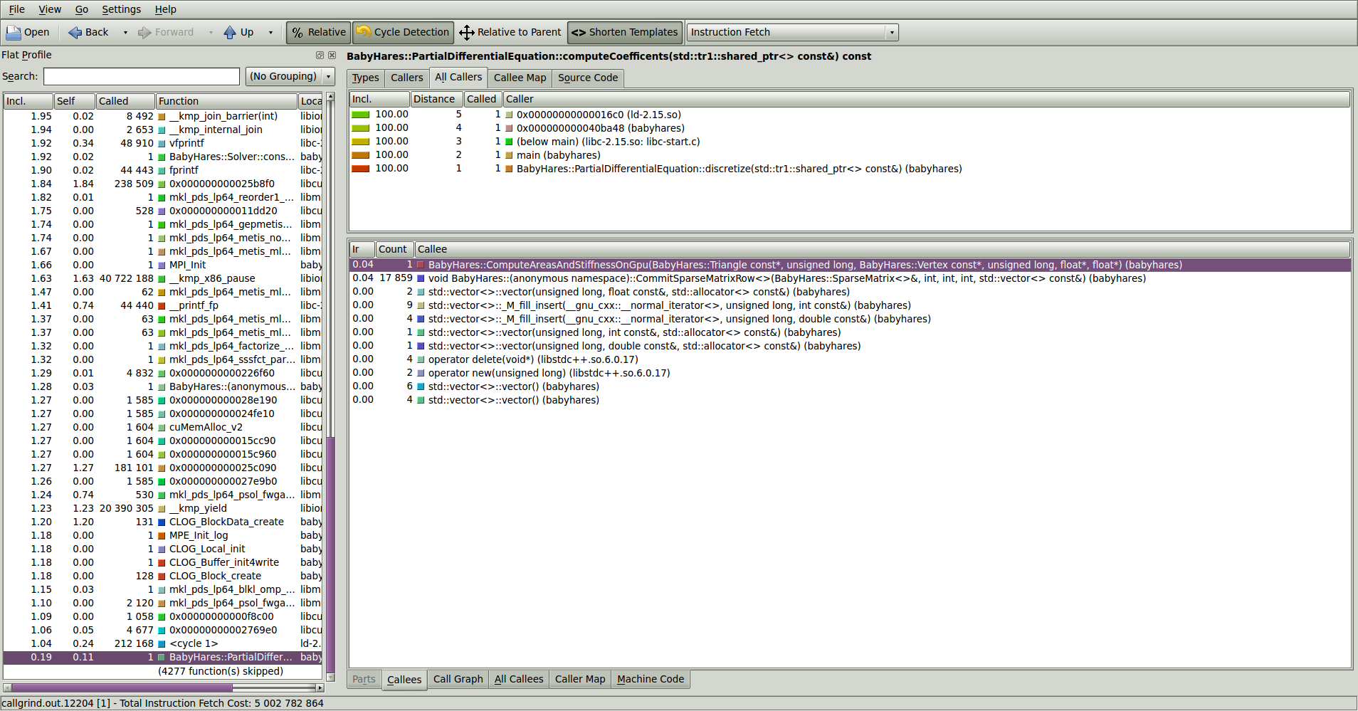
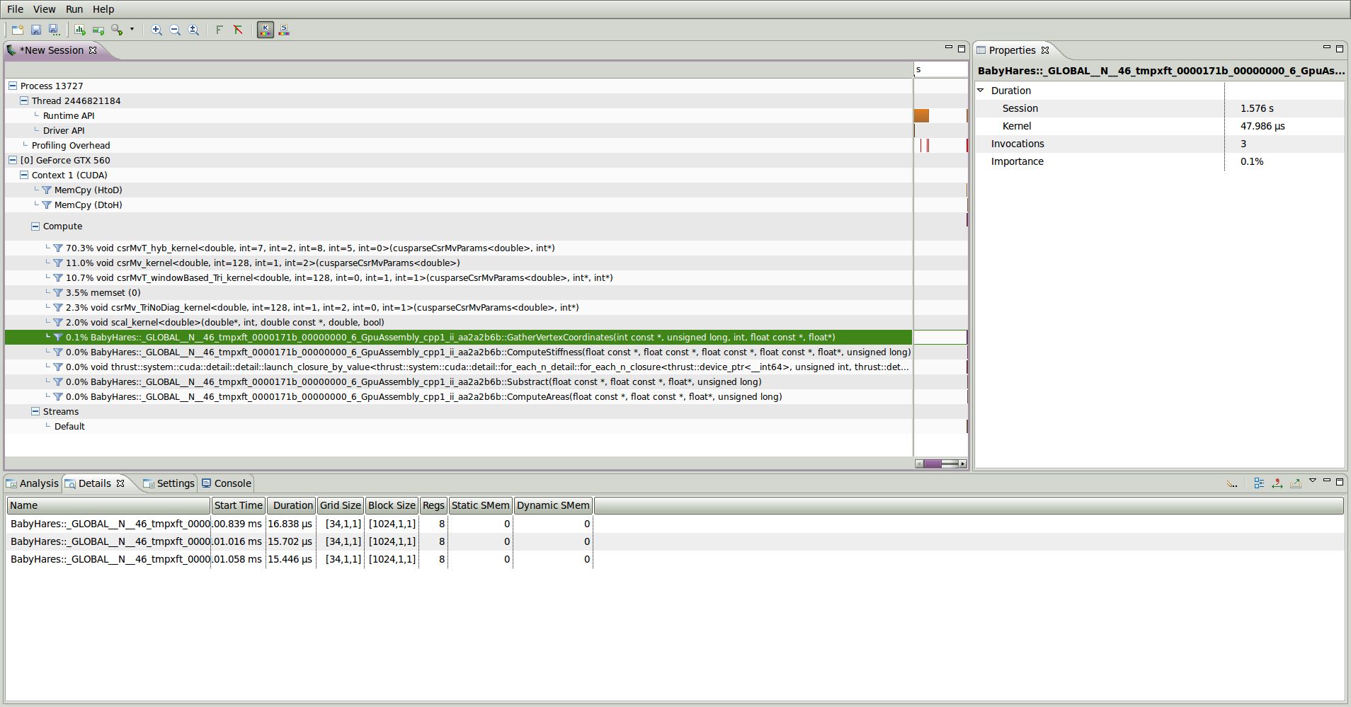
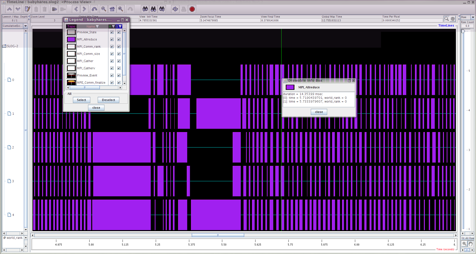
I spent some time playing with kcachegrind (general perf), nvvp (GPU perf) and jumpshot (MPI perf).
kcachegrind


nvvp


MPE
Conclusion
That’s all for this “mini” post. It covered quite a few HPC related technologies. I will discuss performnance and optimization in another post. In the next post I will modify the solver to handle the linear mild-slope equation as I promised. It’s going to be quite involved this time.
blog comments powered by Disqus