The Lyttelton port wave penetration project: Part 1

In this series of mini-posts, I will try to create a wave penetration simulator, a baby version of HARES.

For this kickoff post I will focus on retrieving the Lyttelton port geometry, generate a mesh, partition it into more than two subdomains (5 for example) and modify the Perl scripts we used in the first Schur complement post in order to deal with many subdomains. I will also demonstrate how we can use the Google Maps JavaScript API, the OpenStreetMap tiles as well as WebGL to display the mesh and the sudomains.

Retrieving the port geometry

Raw data

I will retrieve the Lyttelton port geometry from the OSM data using the Overpass API and taking advantage of the coastline tag.

Here is the query I’m using the get the coastline nearby the Lyttelton port:

 1 <osm-script output="xml">
 2   <query type="way">
 3    <has-kv k="natural" v="coastline"/>
 4    <bbox-query
 5     w="172.70914950376547" s="-43.611191483302505"
 6     e="172.72557535177208" n="-43.60308883447627"/>
 7   </query>
 8  <print mode="meta"/>
 9  <recurse type="down"/>
10  <print mode="meta" order="quadtile"/>
11 </osm-script>

Let’s run it in an Overpass sandbox:

View Larger Map

As you can see the query is returning too much coastline.

Here is the exported data in the OSM XML file format:

• Raw Lyttleton port coastline

Open boundary

The next stage is to cleanup unwanted edges and close the geometry with an open boundary. An open boundary is not a physical boundary. The condition on the open boundary will be discused at a later stage.

In order to do so, I’m using the josm editor.

Here is the final geometry in the OSM XML file format:

• Lyttleton port with open boundary

It’s worth noticying that manually added nodes are flaged with an action='modify' tag by the editor:

<node id='-2498' action='modify' visible='true' lat='-43.613555333973856' lon='172.71590659752025' />

I will take advantage of this in order to distinguish between closed and open boundaries later on.

Conclusion

I’m done with this part. Note that the current geometry is currently in “latitude/longitude” space. Next stage is to generate a mesh.

Mesh generation

In this part I’m going to use bamg, which is shiped with the Metis software I demonstrated in the first post. Given a geometry, bamg will generate a mesh using sophisticated algorithm.

I must convert the OSM file into the bamg mesh file format.

One thing we have to take care of is to project the geometry from “lat/lon” space to Mercator space and then make the projected geometry dimensionless.

Here is a script doing that:

 1 #! /usr/bin/perl
 2 use strict;
 3 use warnings;
 4 use XML::XPath;
 5 use Math::Trig 'pi';
 6 use List::Util 'min' ,'max';
 7 
 8 use Geo::Proj4;
 9 my $proj = Geo::Proj4->new(init => "epsg:3857") or die;
10 
11 my $osm = XML::XPath->new(filename => 'lyttelton.osm');
12 my $nodeset = $osm->find('/osm/node');
13 
14 my $bamgid = 0;
15 my %nodes;
16 
17 my $xmin = 'inf';
18 my $xmax = '-inf';
19 my $ymin = 'inf';
20 my $ymax = '-inf';
21 
22 my $earthRadius = 6378137;
23 
24 foreach my $node ($nodeset->get_nodelist) {
25   ++$bamgid;
26     my $osmid = $node->getAttribute("id");
27     my $lat = $node->getAttribute("lat");
28     my $lon = $node->getAttribute("lon");
29     my $vnode = $node->getAttribute("action");
30 
31     # EPSG 3857 projection
32     my ($x,$y) = $proj->forward($lat, $lon);
33 
34     # Google mercator convertion
35     $x = 256 * (0.5 + $x / (2 * pi * $earthRadius));
36     $y = 256 * (0.5 - $y / (2 * pi * $earthRadius));
37 
38     $xmin = min($x,$xmin);
39     $xmax = max($x,$xmax);
40         
41     $ymin = min($y,$ymin);
42     $ymax = max($y,$ymax);
43 
44     $nodes{$osmid} = [$bamgid, $x, $y, $vnode];
45 }
46 
47 # Make the geometry dimensionless
48 my $d = max($xmax - $xmin, $ymax - $ymin);
49 foreach my $node (values(%nodes)) {
50     $node->[1] = ($node->[1] - $xmin) / $d;
51     $node->[2] = ($node->[2] - $ymin) / $d;
52 }
53 
54 # Remember these in order to display on top of a Google map later on
55 print "Translate: ($xmin, $ymin)\n";
56 print "Scale:$d\n";
57 
58 # Create bamg input file
59 open my $out, "> lyttelton_0.mesh";
60 print $out "MeshVersionFormatted 1\n\n";
61 print $out "Dimension 2\n\n";
62 print $out "Vertices " . $bamgid . "\n";
63 
64 foreach my $node (sort {$a->[0] <=> $b->[0]} values(%nodes)) {
65   printf $out  "%.12f %.12f 1\n", $node->[1], $node->[2];
66 }
67 
68 my $edgeset = $osm->find('/osm/way/nd');
69 
70 print $out "\nEdges " . ($edgeset->size - 1) . "\n";
71 
72 my $start = 0;
73 
74 foreach my $edge ($edgeset->get_nodelist) {
75     my $end = $edge->getAttribute("ref");
76     if ($start != 0) {
77       my $boundaryId = $nodes{$start}->[3] || $nodes{$end}->[3] ? 2 : 1;
78       print $out $nodes{$start}->[0] ." " . $nodes{$end}->[0] . " " . $boundaryId . "\n";
79     }
80     $start = $end;
81 }

Here is the bamg input:

• Lyttelton geometry for bamg

Here is the command line for bamg:

bamg  -g lyttelton_0.mesh -coef 0.06  -ratio 20 -o lyttelton.mesh

And here is the generated mesh file:

• Lyttelton mesh

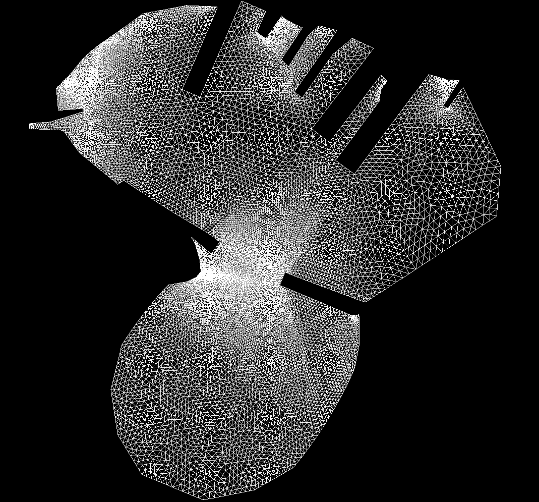
This is what a Lyttelton port small mesh looks like:

Conclusion

It seems quite easy to use the OSM data for baby coastal engineering. I’m missing the water depth inside the port though: I will address this in another post (3rd one). In the next stage we will decompose the generated mesh into 5 subdomains.

Partitioning

To make this project more challenging, I will implement a parallel solver. In order to do so I will apply domain decomposition techniques. I detailed the partioning tools and the methodology in the first Schur complement post so that this part is going to be concise.

• Metis input graph : lyttelton.metis_graph
• Metis output element partition : lyttelton.metis_graph.epart.5
• Metis output vertex partition : lyttelton.metis_graph.npart.5

That’s it.

Interface computation and unknown reordering

One last thing we have to do is to compute the domains interface and reorder the interface unknowns to improve the sparsity pattern of the “interface-interface” stiffness matrix. Again I addressed this in the first Schur complement post, but only for the two subdomains case. I had to slightly modify the scripts in that post to make them work for many subdomains.

Here are the modifications on github:

• Find the interface for many subdomains
• Reorder the unknowns for many subdomains

Ultimately here is the interface:

• interface2.vids

Visualization

So here we are ! Ready to display our domain and subdomains on top of the matching OSM tiles thanks to the Google Maps JavaScript API and WebGL:

View Larger Map

Conclusion

In the next mini-post, I will implement several parallel versions of the “trace first” Schur complement method applied to the data I generated using MPI.