The Schur Complement Method: Part 1
This post is going to illustrate the primal Schur complement method briefly described here. The Schur complement method is a strategy one can use to divide a finite element problem into independant sub-problems. It’s not too involved but requires good understanding of block Gaussian elimination, reordering degrees of freedom plus a few “tricks of the trade” to avoid computing inverse of large sparse matrices.
A (finite element) problem
In that part, we’re going to create all the data needed to implement the method:
- a mesh
- a system of linear equations
A 2D Poisson’s equation
First step is to choose a problem. For example, solve a Poisson equation.
Given a domain \(\Omega\), the problem is to find \(\varphi\) such that
I chose a L-shape for \(\Omega\):
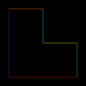
FreeFem++
Since this post doesn’t aim to illustrate in great details the finite element method itself, I’m going to translate the weak formulation of the problem into the FreeFem++ language. What FreeFem++ is going to do for us is to create the desired mesh and system of linear equations.
The weak formulation of the problem is to find \(u\) such that \(\int_\Omega \left( \frac{\partial u}{\partial x}\frac{\partial v}{\partial x} + \frac{\partial u}{\partial y}\frac{\partial v}{\partial y} \right)dxdy + \int_\Omega vdxdy = 0, \forall v\).
Note that I will be using Lagrange P1 elements to make reordering of the degrees of freedom (DoF) easier in the next step.
This is how the problem translates into the FreeFem++ langage:
 1 // Describe the geometry of the domain
 2 border red(t=0,1){x=t;y=0;};
 3 border green(t=0,0.5){x=1;y=t;};
 4 border yellow(t=0,0.5){x=1-t;y=0.5;};
 5 border blue(t=0.5,1){x=0.5;y=t;};
 6 border orange(t=0.5,1){x=1-t;y=1;};
 7 border violet(t=0,1){x=0;y=1-t;};
 8
 9 // Build a mesh over that domain
10 mesh Th = buildmesh (red(6) + green(4) + yellow(4) + blue(4) + orange(4) + violet(6));
11
12 // Define the finite element space, using Lagrange P1 element
13 fespace Vh(Th,P1);
14
15 // Define u, the function we are looking for, as well as v, the test function in the weak formulation.
16 Vh u=0,v;
17
18 // Define the value of the Laplacian of phi within the domain
19 func f= 1;
20
21 // Define the value of phi on the border of the domain
22 func g= 0;
23
24 // Describe the problem using the weak formulation
25 problem Poisson2D(u,v) =
26     int2d(Th)(dx(u)*dx(v) + dy(u)*dy(v)) // First integral
27   + int2d(Th) (v*f)  // Second integral
28   + on(red,green,yellow,blue,orange,violet,u=g); // What happens on the border
Given that script, FreeFem++ is going to:
- build a mesh;
- build a system of linear equations: a square matrix
\(A\)and a column vector\(b\). Each DoF (unknown) is the value of the function we are looking for at a given vertex of the mesh (because we choosed Lagrange P1 elements).
Hereafter is the mesh (built by FreeFem++) I am going to work with in the next steps:
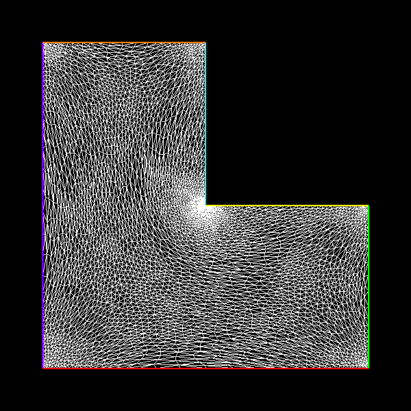
It is made of 7215 triangles and 3735 vertices.
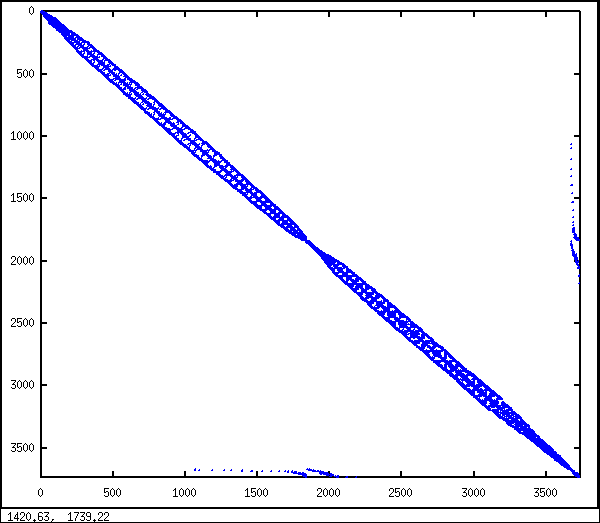
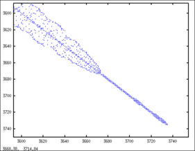
Hereafter is the sparsity pattern of the corresponding \(A\) matrix:
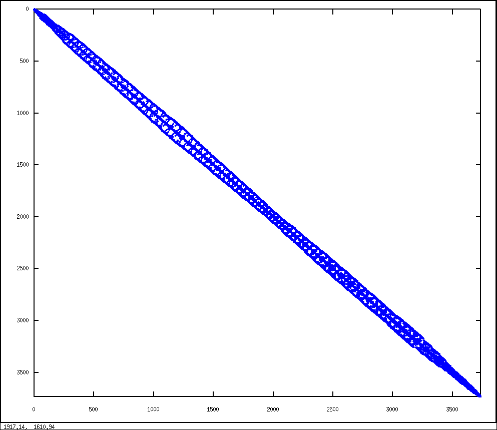
Its size is 3735x3735. It’s a band matrix because of the way FreeFem++ numbered the DoF.
Conclusion and spoiler
So there we are, we got all the data needed to get started. What needs to be done next is:
- partition the domain
- reorder the DoF
- implement the method itself
- celebrate
By the way, if you want to have a look at the solution to the problem, click here
Partitioning the domain
The next stage to illustrate the method is to partition the initial domain into two sub-domains. In order to do so, one can use specialized tools such as Chaco or Metis. I’m arbitrarily going to use Metis.
Metis
Metis input is a graph and a number of sub-domains. It doesn’t use the coordinates of the vertices. I generated Metis input graph from the mesh using this one liner:
perl -ne 'push @T, "$1 $2 $3\n" if /(\d+) (\d+) (\d+) (\d+)/; END{print @T."\n"; print for @T}' poisson2D.mesh > poisson2D.metis_graphThe command mpmetis poisson2D.metis_graph 2 will output two files:
poisson2D.metis_graph.epart.2 (respectively poisson2D.metis_graph.npart.2) contains the domain indices (starting from 0) of each
triangle (respectively vertex) of the mesh. For example, line 42 of poisson2D.metis_graph.epart.2 will contain a 0 if triangle number
42 belongs to the domain number 0.
Identifying the boundary vertices
Sadly, the Metis output doesn’t tell us what are the boundary vertices so that we need to do a little bit of post-processing.
Remember that we need to identify the boundary DoFs to pack them into a single matrix block in a later stage.
The script hereafter is going to fan out vertices ids into separate files,domain1.vids (vertices within domain 1 exclusively), domain2.vids and interface.vids (vertices on the interface).
 1 #! /usr/bin/perl
 2 use strict;
 3 use warnings;
 4
 5 open my $FDTRIANGLES, "poisson2D.metis_graph";
 6 open my $FDIDS, "poisson2D.metis_graph.epart.2";
 7
 8 my @vertexToDomain;
 9 my %interface;
10
11 while (<$FDTRIANGLES>) {
12 	if (/(?<vid1>\d+) (?<vid2>\d+) (?<vid3>\d+)/) {
13 		my $domain = <$FDIDS> + 1;
14 		CheckVertex($+{vid1}, $domain);
15 		CheckVertex($+{vid2}, $domain);
16 		CheckVertex($+{vid3}, $domain);
17 	}
18 }
19
20 my @DOMAINFD;
21 open $DOMAINFD[1], "> domain1.vids";
22 open $DOMAINFD[2], "> domain2.vids";
23 open my $INTERFACEFD, "> interface.vids";
24 while (my ($vid, $domain) = each @vertexToDomain) {
25 	next if !$vid;
26 	my $fd = exists $interface{$vid} ? $INTERFACEFD : $DOMAINFD[$domain];
27 	print $fd $vid."\n";
28 }
29
30 # Count the number of domain a vertex belongs to, if it's greater than 1
31 # that vertex is on the interface
32 sub CheckVertex {
33 	my ($vid, $domain) = @_;
34 	if ($vertexToDomain[$vid] && $vertexToDomain[$vid] != $domain) {
35 		$interface{$vid}++;
36 	} else {
37 		$vertexToDomain[$vid] = $domain;
38 	}
39 }Conclusion
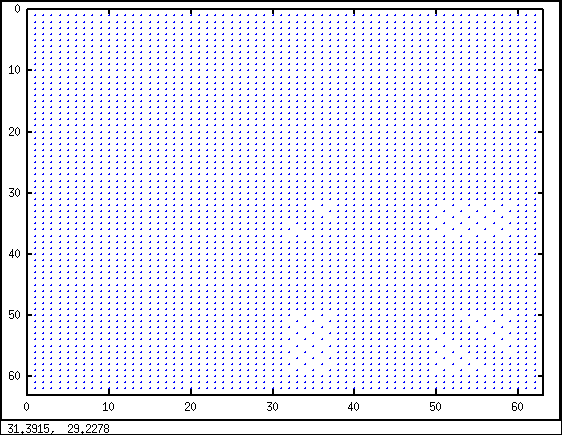
Finally, here is what the partition looks like:
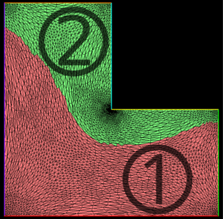
Domains 1 and 2 respectively contain 1839 and 1834 DoFs. The interface contains 62 DoFs. Tools such as Metis are doing a good job at balancing the size of the sub-domains while minimizing the size of the interfaces.
Reordering the degrees of freedom
Now that I partitioned the domain, we have everything needed to give the sytem of linear equations the structure needed by the Schur complement method:
where
\(A_{ii}\)is the block coupling the interior of domain\(i\)to itself;\(A_{\Gamma\Gamma}\)is the block coupling the interface to itself;\(A_{\Gamma i}\)is the block coupling the interface to the interior of domain\(i\);\(A_{i\Gamma}\)is the block coupling the interior of domain\(i\)to the interface
Octave
From now on, I will be using Octave.
To do the reordering I’m going to create a permutation matrix \(P\) out of the domain1.vids, domain2.vids and interface.vids and apply it to \(A\) (\(PAP^\top\)) and \(b\) (\(Pb\)) from the first step.
1 load("-ascii", "domain1.vids");
2 load("-ascii", "domain2.vids");
3 load("-ascii", "interface.vids");
4 q = [domain1; domain2; interface];
5 A = A(q,q);
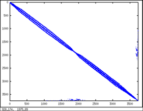
6 b = b(q);Hereafter is the spy of the desired block matrix after applying the permutation:
Matrix pr0n:
\(A_{11}\), \(A_{22}\) sparsity patterns are similar to the initial \(A\) matrix one since we took care of preserving the relative order
of DoFs in the interior of the domains.
\(A_{11}\): 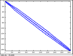
\(A_{22}\): 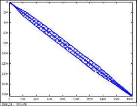
However \(A_{TT}\) sparsity pattern doesn’t look great considering that the geometry here is a simple polyline. The initial DoF ordering
does not make sens on the interface. I’m going to address this in the next section.
\(A_{TT}\): 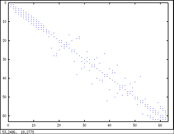
\(A_{T1}\): 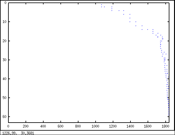
\(A_{T2}\): 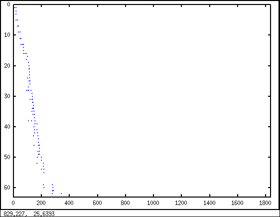
\(A_{TT}\) reloaded
I’m going to improve \(A_{TT}\) sparsity pattern.
The idea is to walk the interface from one end to the other, dumping DoF ids as we go.
This new permutation is going to preserve locality and will greatly improve the sparsity pattern of \(A_{TT}\).
  1 #! /usr/bin/perl
  2 use strict;
  3 use warnings;
  4
  5 open my $FDTRIANGLES, "poisson2D.metis_graph";
  6 open my $FDIDS, "poisson2D.metis_graph.epart.2";
  7
  8 my %triangleToVertices;
  9 my %vertexToTriangles;
 10 my %interface;
 11 my %interfaceGraph;
 12
 13 open my $INTERFACEFD, "interface.vids";
 14 while (<$INTERFACEFD>) {
 15 	$interface{int($_)}++;
 16 }
 17
 18 # Build connectivity and reverse connectivity tables for
 19 # domain 1 elements on the interface
 20 my $triangleId = 0;
 21 while (<$FDTRIANGLES>) {
 22 	if (/(?<vid1>\d+) (?<vid2>\d+) (?<vid3>\d+)/) {
 23 		++$triangleId;
 24 		my $domain = <$FDIDS> + 1;
 25 		if ($domain == 1) {
 26 			AddVertices($triangleId, $1, $2, $3);
 27 			AddTriangle($+{vid1}, $triangleId);
 28 			AddTriangle($+{vid2}, $triangleId);
 29 			AddTriangle($+{vid3}, $triangleId);
 30 		}
 31 	}
 32 }
 33
 34 # Go through each edge and check if it's on the interface
 35 while (my ($tid, $vids) = each %triangleToVertices) {
 36 	for (0..$#{$vids}) {
 37 		my ($vid1, $vid2) = @{$vids}[$_, ($_ + 1) % @{$vids}];
 38 		if (IsInterfaceEdge($vid1, $vid2)) {
 39 			AddInterfaceEdge($vid1, $vid2);
 40 		}
 41 	}
 42 }
 43
 44 # Walk the interface
 45 my $start = FindInterfaceEnd();
 46 WalkInterface($start, $start);
 47
 48 sub AddVertices {
 49 	my ($tid, $vid1, $vid2, $vid3) = @_;
 50 	if (exists $interface{$vid1} || exists $interface{$vid2} || exists $interface{$vid3}) {
 51 		$triangleToVertices{$tid} = [$vid1, $vid2, $vid3];
 52 	}
 53 }
 54
 55 sub AddTriangle {
 56 	my ($vid, $tid) = @_;
 57 	if (exists $interface{$vid}) {
 58 		$vertexToTriangles{$vid}{$tid}++;
 59 	}
 60 }
 61
 62 sub AddInterfaceEdge {
 63 	my ($vid1, $vid2) = @_;
 64 	$interfaceGraph{$vid1}{$vid2}++;
 65 	$interfaceGraph{$vid2}{$vid1}++;
 66 }
 67
 68 # An interface edge has its two vertices on the interface
 69 # and belongs to one and only one domain 1 triangle.
 70 sub IsInterfaceEdge {
 71 	my ($vid1, $vid2) = @_;
 72
 73 	return 0 unless exists $interface{$vid1} && exists $interface{$vid2};
 74
 75 	my @tids1 = keys %{$vertexToTriangles{$vid1}};
 76 	my @tids2 = keys %{$vertexToTriangles{$vid2}};
 77
 78 	my %union;
 79 	my $triangleCount = 0;
 80 	for my $tid (@tids1, @tids2) {
 81 		if (++$union{$tid} == 2) {
 82 			$triangleCount++;
 83 		}
 84 	}
 85
 86 	return $triangleCount == 1;
 87 }
 88
 89 # The interface should have two ends.
 90 # An end is simply a vertex connected to only one other vertex.
 91 sub FindInterfaceEnd {
 92 	while (my ($from, $tos) = each %interfaceGraph) {
 93 		if (keys %{$tos} == 1) {
 94 			return $from;
 95 		}
 96 	}
 97 	exit -1;
 98 }
 99
100 # Perform a simple DFS to walk the interface
101 # and print the vertex ids as we go.
102 sub WalkInterface {
103 	my ($u, $v) = @_;
104 	print $v."\n";
105 	for (keys %{$interfaceGraph{$v}}) {
106 		next if $_ == $u;
107 		return WalkInterface($v, $_);
108 	}
109 }And … voila:
\(A_{TT}\): 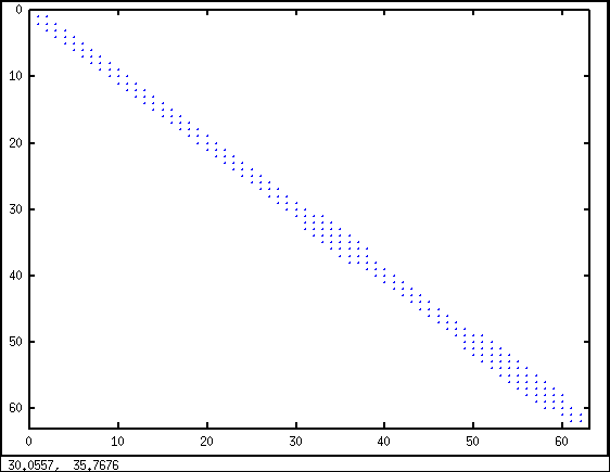
If you’re wondering how can one interface DoF be coupled to 4 other DoFs, this happens when one interface DoF belongs to 2 triangles and each of these triangles has all its vertices on the interface.
Conclusion
We’re done doing the reordering. Here is the final version:
We’re now ready to define a few more variables in Octave:
 1 i1 = length(domain1);
 2 i2 = i1 + length(domain2);
 3
 4 A11 = AA(1:i1, 1:i1);
 5 A1T = AA(1:i1, i2+1:end);
 6 A22 = AA(i1+1:i2, i1+1:i2);
 7 A2T = AA(i1+1:i2, i2+1:end);
 8 AT1 = AA(i2+1:end, 1:i1);
 9 AT2 = AA(i2+1:end, i1+1:i2);
10 ATT = AA(i2+1:end, i2+1:end);
11 U = zeros(length(A), 1);
12 clear A;
13
14 F1 = F(1:i1);
15 F2 = F(i1+1:i2);
16 FT = F(i2+1:end);
17 clear F;
Solving on the interface
Block Gaussian elimination
Being able to solve first for the interface without even considering what’s happening in the interior of the subdomains
might seem magical: this is nothing more than block Gaussian elimination applied to the matrix we crafted
in the previous stages. In \(\eqref{eq:mainsystem}\), multiply the first line by \(A_{T1}A_{11}^{-1}\), the second line by \(A_{T2}A_{22}^{-1}\),
substract both quantities from the third line and you end up with:
In other words, we need to solve:
where \(\Sigma = A_{TT} - A_{T1}A_{11}^{-1}A_{1T} - A_{T2}A_{22}^{-1}A_{2T}\)
and \(\tilde{b} = F_{T} - A_{T1}A_{11}^{-1}F_{1} - A_{T2}A_{22}^{-1}F_{2}\)
Schur complement
In the numerical analysis lingo, \(\Sigma\) is known as the Schur complement of \(A_{TT}\) in \(A\).
As we can see, both \(\Sigma\) and \(\tilde{b}\) depend on \(A_{11}^{-1}\) and \(A_{22}^{-1}\).
However, \(A_{11}\) and \(A_{22}\) are large matrices we should try not to invert.
Anyway, let’s explicitely compute the Schur complement for our baby problem and have a look:
1 % Bad bad bad !
2 spy(ATT - AT1 * inv(A11) * A1T + AT2 * inv(A22) * A2T);
It’s crazy dense!
Furthermore Octave tells us that \(A_{11}\) and \(A_{22}\) are singular to machine precision:
warning: inverse: matrix singular to machine precision, rcond = 1.65116e-30
Iterative method
To summarize we would like to avoid:
- explicitely computing
\(\Sigma\)in order to solve\(\eqref{eq:interfacesystem}\); - explicitely inverting
\(A_{11}\)or\(A_{22}\)
If we try to satisfy these two constraints, it is clear that we can’t use a direct method to solve \(\eqref{eq:interfacesystem}\).
On the other hand, if we choose an iterative method such as the preconditioned conjugate gradient method (PCG),
we just need to mulitply, each iteration of the method, a current solution \(u\) by \(\Sigma\). Multiplying by \(\Sigma\) is
a different story than explicitely computing \(\Sigma\):
Decoupled Dirichlet problems
I’m now going to describe a simple tactic to evaluate \(A_{11}^{-1}A_{1T}u\) and \(A_{22}^{-1}A_{2T}u\) without inverting \(A_{11}\) and \(A_{22}\).
Assume you’re given a very large invertible matrix \(A\) and one (1) vector \(b\) and you’re tasked to compute the quantity \(A^{-1}b\).
Would you explicitely compute \(A^{-1}\) ?
Probably not.
What you would do instead is to find \(x\) such that \(Ax=b\).
Then \(x=A^{-1}b\), which is what you were tasked to compute.
Following this idea, I’m going to use a direct method to compute these quantities: I will compute the LU decomposition of \(A_{11}\) (respectively \(A_{22}\)) once and for all, and every PCG iteration, compute \(b = A_{1T} * u\) (respectively \(b = A_{2T} * u\)) and solve \(A_{11}x=b\) (respectively \(A_{22}x=b\)). The same tactic is used to compute \(A_{11}^{-1}F_{1}\) and \(A_{22}^{-1}F_{2}\) in \(\tilde{b}\).
Each iteration of the PCG, we end up solving decoupled Dirichlet problems on each domain.
All together, this looks like this:
1 [L11, U11, p11, q11] = lu(A11, 'vector');
2 q11t(q11) = 1:length(q11);
3 clear A11;
4 clear q11;
5
6 [L22, U22, p22, q22] = lu(A22, 'vector');
7 q22t(q22) = 1:length(q22);
8 clear A22;
9 clear q22;
10
11 FT -= AT1 * (U11 \ (L11 \ F1(p11)))(q11t) ...
12 + AT2 * (U22 \ (L22 \ F2(p22)))(q22t);
13
14 U(i2+1:end) = pcg(@(x) ...
15 ATT * x ...
16 - AT1 * (U11 \ (L11 \ (A1T * x)(p11)))(q11t) ...
17 - AT2 * (U22 \ (L22 \ (A2T * x)(p22)))(q22t), FT, 1.e-9, 200);
18
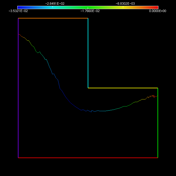
19 clear ATT;
20 clear FT;Solution on the interface:
Conclusion
I think the method in this post is along the lines of what was described in the wikipedia article:
The important thing to note is that the computation of any quantities involving
\(A_{11}^{-1}\)or\(A_{22}^{-1}\)involves solving decoupled Dirichlet problems on each domain, and these can be done in parallel. Consequently, we need not store the Schur complement matrix explicitly; it is sufficient to know how to multiply a vector by it.
Note that it is not the only method.
Solving on the subdomains
Once we computed \(U_{T}\), the solution on the interface, we can quickly solve in parallel for \(U_{1}\) and \(U_{2}\) as we already computed the LU decomposition of both \(A_{11}\) and \(A_{22}\).
Subdomain 1
First line of \(\eqref{eq:mainsystem}\) gives us
1 U(1:i1) = (U11 \ (L11 \ (F1 - A1T * U(i2+1:end))(p11)))(q11t);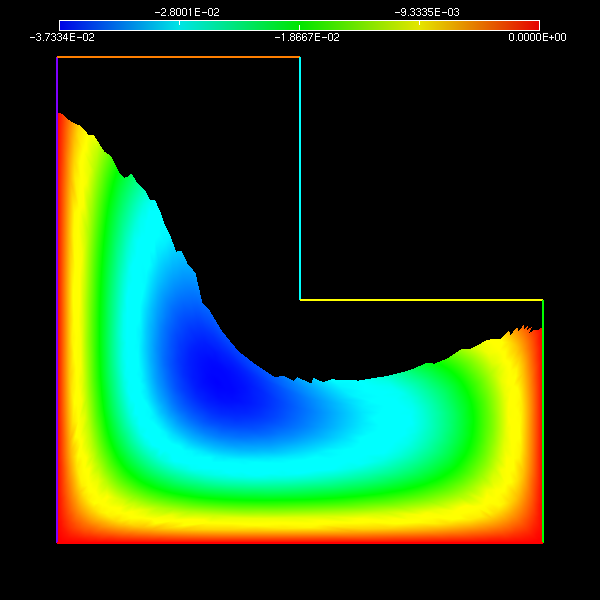
Subdomain 2
Similarly, second line of \(\eqref{eq:mainsystem}\) gives us
1 U(i1+1:i2) = (U22 \ (L22 \ (F2 - A2T * U(i2+1:end))(p22)))(q22t);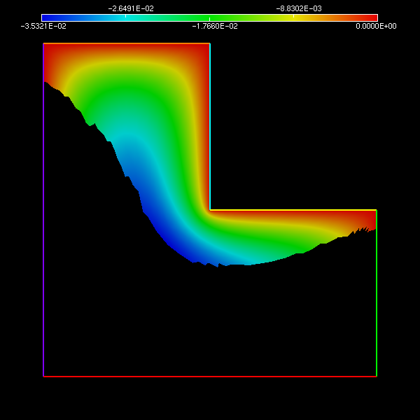
Ultimately we need to revert ordering of the DoFs to display the solution:
1 % Reorder back DoFs
2 p(q) = 1:length(q);
3 U = U(p);
Fusiiiiiiiiiiiiion !
Boum \o/

Conclusion
Hopefully, you now have a good overview of how one can implement the Schur complement method. I also hope that it wasn’t too boring and that you’re going to reuse that knowledge for your own projects. I didn’t talk about implementing the method for more than 2 subdomains, preconditioning, parallel implementation, &c. Another time.
In the next episode
In the next episode, “The Schur Complement Method: Part 2”, I’m going to describe … the DUAL Schur complement method. It’s going to be a little more involved but not that much.
blog comments powered by Disqus