The alternator simulation project

In this post I’m going to illustrate how to implement a finite element simulation of an alternator in motion coupled to a linear electrical circuit.

The simulation computes the magnetic vector potential within a (2D) radial cross section of the machine I’m about to describe.

Here’s an example for a 3000rpm rotor speed and a stator energized with a 50Hz AC current:

View Larger Simulation

The code is here

Description of the machine

The machine we’re going to study is an unusual induction generator of the squirel-cage type.

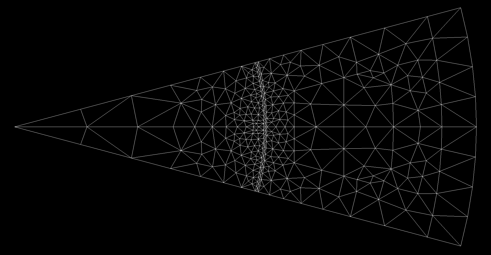
This is \(1/12^{th}\) of the machine:

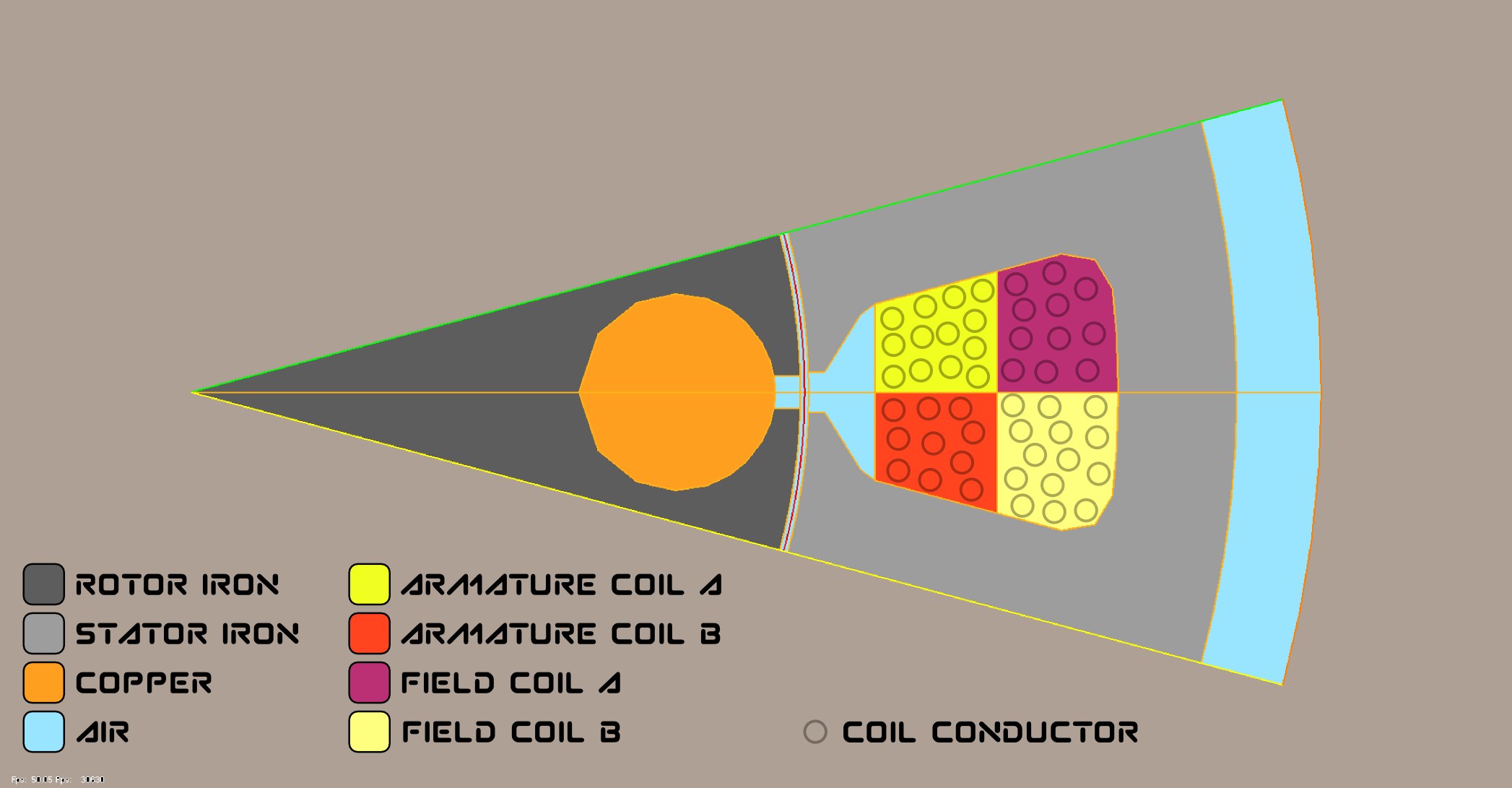
The rotor has 12 massive coper rods shorted by rings at both ends: the so called squirel cage. Rods are enclosed in a cyclinder made of iron laminations.

The stator, made of iron laminations too, has 12 winding slots. The winding pattern is as follow:

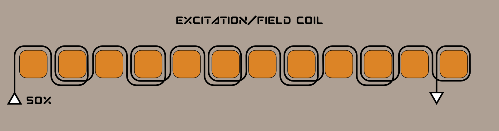
Notice that the field coil goes up/up, down/down, up/up … This will be very important later on when computing the current density in the coils.

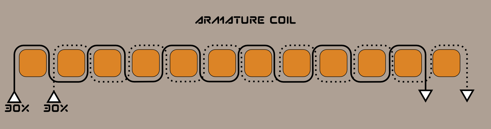
Again, notice that the armature coil goes up/down when the field coil goes up/up, and then down/up, up/down …

The diameter of the machine is 80mm, its depth/thickness is 50mm.

Modelization

Periodicity

Because of the problem periodicity, we can reduce the ammount of computation by modeling only a slice of the machine.

To find the size of the smallest possible slice we compute the greatest common divisor (\(gcd\)) of the number of rods and slots and only simulate a \(360 / gcd\) degrees machine slice.

Next, in order to decide if we need to use periodic or anti-periodic boundary conditions to join our alternator slices, we simply observe that if we apply Kirchoff current’s law to the rotor squirel cage topology, the eddy currents flowing through one rod will flow in the opposite direction in the previous and next rods so that we use periodic (respectively anti-periodic) boundary condition if the slice contains an even (respectively odd) number of rod.

It comes that for this particular endeavour we can simulate \(1/12^{th}\) of the machine (30 degrees), so a single rod and a single slot, and must use anti-periodic boundary condition.

When implementing the finite element method using first order Lagrange element to solve non periodic problem we have a one to one mapping between mesh vertices and degrees of freedom (\(dof\)) so that we can identify vertices with \(dof\).

For example a single quadrangular first order Lagrange element has 4 vertices and leads to a 4 \(dof\) stiffness matrix:

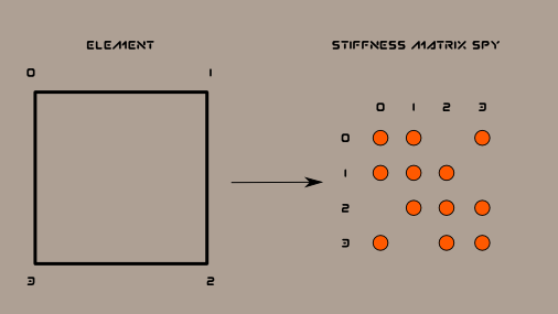
However if we consider an (anti-)periodic along one axis element, it leads to a 2 \(dof\) stiffness matrix:

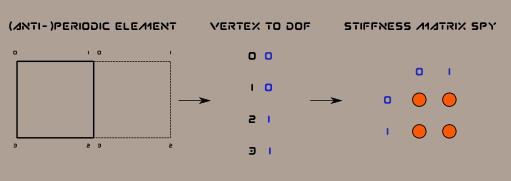
We can also illustrate further what’s going on by writing the equations:

$$\begin{aligned} & \begin{pmatrix} a_{0,0} & a_{0,1} & a_{0,2} & a_{0,3}\\\ a_{1,0} & a_{1,1} & a_{1,2} & a_{1,3}\\\ a_{2,0} & a_{2,1} & a_{2,2} & a_{2,3}\\\ a_{3,0} & a_{3,1} & a_{3,2} & a_{3,3} \end{pmatrix} \begin{pmatrix} x_0\\\ x_1\\\ x_2\\\ x_3 \end{pmatrix} = \begin{pmatrix} b_0 \\\ b_1 \\\ b_2 \\\ b_3 \end{pmatrix}\\\ \Leftrightarrow & \begin{pmatrix} a_{0,0} & a_{0,1} & a_{0,2} & a_{0,3}\\\ a_{0,1} & a_{1,1} & a_{1,2} & a_{1,3}\\\ a_{0,2} & a_{1,2} & a_{2,2} & a_{2,3}\\\ a_{0,3} & a_{1,3} & a_{2,3} & a_{3,3} \end{pmatrix} \begin{pmatrix} x_0\\\ \pm x_0\\\ x_2\\\ \pm x_2 \end{pmatrix} = \begin{pmatrix} b_0 \\\ b_1 \\\ b_2 \\\ b_3 \end{pmatrix}, x_1 = \pm x_0, x_3 = \pm x_2 \text{, as per stiffness matrix symmetry and element periodicity}\\\ \Leftrightarrow & \begin{pmatrix} a_{0,0} \pm a_{0,1} & a_{0,2} \pm a_{0,3}\\\ a_{0,1} \pm a_{1,1} & a_{1,2} \pm a_{1,3}\\\ a_{0,2} \pm a_{1,2} & a_{2,2} \pm a_{2,3}\\\ a_{0,3} \pm a_{1,3} & a_{2,3} \pm a_{3,3} \end{pmatrix} \begin{pmatrix} x_0\\\ x_2 \end{pmatrix} = \begin{pmatrix} b_0 \\\ b_1 \\\ b_2 \\\ b_3 \end{pmatrix}, x_1 = \pm x_0, x_3 = \pm x_2\\\ \Leftrightarrow & \begin{pmatrix} a_{0,0} \pm 2 a_{0,1} + a_{1,1} & a_{0,2} \pm a_{0,3} \pm a_{1,2} + a_{1,3}\\\ a_{0,2} \pm a_{0,3} \pm a_{1,2} + a_{1,3} & a_{2,2} \pm 2 a_{2,3} + a_{3,3} \end{pmatrix} \begin{pmatrix} x_0\\\ x_2 \end{pmatrix} = \begin{pmatrix} b_0 \pm b_1\\\ b_2 \pm b_3 \end{pmatrix}, x_1 = \pm x_0, x_3 = \pm x_2 \end{aligned}$$

Notice that we also end up with a symmetric linear system.

So that the key to implement (anti-)peridic boundary conditions is to compute the non injective mapping from mesh vertices to \(dof\) as well as introduce a sign/polarity vector in order to remember the sign of each nodal value relative to its \(dof\) (or in short: to deal with all these \(\pm\) in the equations).

• This is how I compute the mapping:

The relevant project class is in https://github.com/ssrb/alternator-fem-webapp/blob/master/domain.ts

• And this is how I assemble the stiffness matrix and load vector using the computed mapping:

The relevant project class is in https://github.com/ssrb/alternator-fem-webapp/blob/master/solver.ts

Motion

In order to simulate the entire machine, we need to match rotor and stator \(dof\) along their common interface. One way to get a match is to first discretize the interface and then use these interface vertices to compute the Delaunay triangulations of both the stator and rotor domains.

How about motion ? Ideally we would like to solve for any rotor/stator angle. That’s doable but a bit too ambitious and we’re instead going to only consider rotations multiple of a fixed “rotation step”. Furthermore we choose a “rotation step” equal to a unit fraction of the domain slice angle, for example \(1/32\) of 30 degrees, so that, by uniformly dividing the interface into 32 segments we can match rotor and stator \(dof\) regardless of the “discrete” rotation angle.

The advantage of this method is that we compute the mesh for both domains once and for all, regardless of the rotation angle.

A drawback of this method is that given the angular speed of the rotor we need to choose the time step of the simulation accordingly. In our example, for a rotor speed of 3000rpm, the time step will be \(60 / (12 * 32 * 3000)\) seconds.

As it rotates, the rotor slice will face both a stator and an “anti-stator” slice. But we won’t explicitly model the anti-stator slice since its nodal values are the opposite of those of the stator slice. Instead we will model a rotor slice which wraps around and use the sign/polarity vector introduced earlier in order to decide if a rotor nodal value is coupled to a stator or “anti-stator” \(dof\).

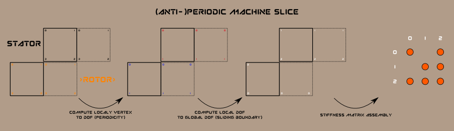
One last thing we need to discuss is how to generate the mapping between rotor/stator “local” \(dof\) to the machine “global” \(dof\):

1. We first map interior “local” \(dof\) for both domains;
2. We then match interface rotor/stator local \(dof\) and assign a single “global” \(dof\) to each pair.

Here is a sketch:

Here is how I compute the mapping:

Relevant project class is in https://github.com/ssrb/alternator-fem-webapp/blob/master/domain.ts

Maxwell’s equations

In this section, I will describe as concisely as I can the derivation of the PDE we’re about to solve.

DISCLAIMER: I’M BY NO MEANS A MAXWELL’S EQUATIONS EXPERT.

Within the machine, the physical quantities we’re intested in, such as magnetic vector potential and current density, are governed by Maxwell’s equations.

• The main equation we’re interested in is the differential form of Ampère’s circuital law which relates the magnetic vector potential \(A\) (V·s·m^-1) to the electric field \(E\) (V·m^-1):

$$\nabla \times \left(\mu \nabla \times A \right) = \sigma E \$$

\(\mu\) (H·m^-1) is the relative magnetic permeability and \(\sigma\) (S·m^-1) the electrical conductivity. In this toy simulation, these quantities are assumed constant for a particular medium (coper, iron, air).

• The next equation we use is the Maxwell–Faraday induction law. It relates the electric field \(E\) to the magnetic vector potential \(A\) and the electric potential \(V\) :

$$E = -\nabla V - \frac{\partial A}{\partial t}$$

Putting these two together we got:

$$\nabla \times \left(\mu \nabla \times A \right) + \sigma \frac{\partial A}{\partial t} = - \sigma \nabla V$$

For this 2D problem \(A\) and \(\nabla V\) are reduced to their z components. That is \(A \equiv \left(0,0,A\right)\) and \(\nabla V \equiv \left(0,0,\partial V / \partial z\right) \).

Now we’re going to make a gross simplification and say that \(\partial V / \partial z \neq 0\) only within the coils. Furthermore, within a coil, we’re going to estimate this quantity as the difference of electric potential at both ends of a single conductor divided by its length:

$$\frac{\partial V}{\partial z} = \frac{V_{z_b} - V_{z_a}}{L}$$

Since the machine is 50mm thick, we set \(L = 0.05\).

Then, using Ohm’s law, we say that:

$$V_{z_a} - V_{z_b} = iR$$

with \(i\) the current going through the coil and \(R\) the resistance of that 50mm long coper conductor. Remember that we care about the sign of \(i\) which depends on the winding pattern.

We can estimate \(R\) using Pouillet’s law:

$$R = \frac{L}{\sigma \mathscr{A}}$$

with \(\mathscr{A}\) the cross-sectional area of the conductor.

Ultimately within a single conductor we got:

$$- \sigma \nabla V \equiv \sigma \frac{V_{z_a} - V_{z_b}}{L} = \sigma \frac{iR}{L} = \sigma \frac{i}{L} \cdot \frac{L}{\sigma \mathscr{A}} = \frac{i}{\mathscr{A}}$$

In the code we estimate the cross-sectional area of a single conductor dividing the cross-sectional area of the entire coil by the number of conductors within the coil.

Putting everything back together we want to solve:

$$\begin{equation}\begin{aligned} \nabla \times \left(\mu \nabla \times A \right) + \sigma \frac{\partial A}{\partial t} = \sum_{k = 1}^{n_{coil}}\psi_k i_k\\\ \psi_k(x) = \begin{cases} \frac{1}{\mathscr{A}_k} \text{ within coil } k\\\ 0 \text{ otherwise} \end{cases} \end{aligned}\label{eq:eq_potential_current}\end{equation}$$

for \(A \equiv \left(0,0,A\right)\) and \(i_k, k = 1 \dots n_{coil}\).

Coupling between magnetic & electrical equations

At this stage we got two unknowns:

• the magnetic vector potential \(A\);
• the currents flowing through the coils \(i_k, k = 1 \dots n_{coil}\)

We are going to get rid of the current.

Admittance matrix

In order to do so we model the linear electrical circuit connected to the machine using a lumped element model: this will give us another relationship between \(A\) and \(i_k, k = 1 \dots n_{coil}\).

The lumped element model of an N port linear electrical circuit can be treated as a single black box whose behavior is concisely described by its admittance parameters:

$$\begin{pmatrix}i_1\\\ \vdots \\\ i_N \end{pmatrix} = Y \begin{pmatrix}v_1\\\ \vdots \\\ v_N \end{pmatrix}$$

where \(v_k, k = 1, \ldots, N\) is the voltage at each port of the circuit.

\(Y\) is called the nodal admittance matrix.

\(Y\) is symmetrical and it is extremely important as if it wasn’t we would not end up with a symmetrical bilinear form later on when trying to solve the PDE.

We can label the ports of the electrical circuit so that:

$$\begin{pmatrix}i_1\\\ \vdots \\\ i_{n_{coil}}\\\ i_{n_{coil} + 1}\\\ \vdots \\\ i_N \end{pmatrix} = \begin{pmatrix} Y_{coils, coils} && Y_{coils, others} \\\ Y_{others, coils} && Y_{others, others} \end{pmatrix} \begin{pmatrix}v_1\\\ \vdots \\\ v_{n_{coil}} \\\ v_{n_{coil} + 1} \\\ \vdots \\\ v_N \end{pmatrix}$$

and since we only care about \(i_k, k = 1, \ldots, n_{coil}\) we write:

$$\begin{cases} \begin{pmatrix}i_1\\\ \vdots \\\ i_{n_{coil}}\end{pmatrix} = I_0 + Y_{coils, coils} \begin{pmatrix}v_1\\\ \vdots \\\ v_{n_{coil}}\end{pmatrix}\\\ I_0 = Y_{coils, others} \begin{pmatrix}v_{n_{coil} + 1} \\\ \vdots \\\ v_N\end{pmatrix} \end{cases}$$

Electromotive force

When the machine is connected to the circuit, the voltage at each port will be equal to the electromotive force \(\mathcal{E}_k\) generated in the matching coil:

$$v_k = \mathcal{E}_k, k = 1, \ldots, n_{coil}$$

As per Lenz’s law:

$$\mathcal{E_k}=-\frac{\partial \Phi_k}{\partial t}$$

where \(\Phi_k\) is the magnetic flux (V·s).

Furthermore

$$\Phi_k = L \int_{\Omega} \psi_k A dx$$

Finally we can rewrite the dextral side of \(\eqref{eq:eq_potential_current}\):

$$\begin{aligned} \sum_{k = 1}^{n_{coil}}\psi_k i_k & = \sum_{k = 1}^{n_{coil}}\psi_k \left( I_{0,k} + \sum_{l = 1}^{n_{coil}} Y_{k.l} v_l\right) \\\ & = \sum_{k = 1}^{n_{coil}}\psi_k \left( I_{0,k} - \sum_{l = 1}^{n_{coil}} Y_{k.l} \frac{\partial \Phi_l}{\partial t} \right) \\\ & = \sum_{k = 1}^{n_{coil}}\psi_k \left( I_{0,k} - L \frac{\partial}{\partial t} \sum_{l = 1}^{n_{coil}} Y_{k,l} \int_{\Omega} \psi_l A dx \right) \end{aligned}$$

and group the vector potential terms on the sinistral side:

$$\begin{equation} \nabla \times \left(\mu \nabla \times A \right) + \sigma \frac{\partial A}{\partial t} + L \frac{\partial}{\partial t} \sum_{k,l = 1}^{n_{coil}} Y_{k,l} \psi_k \int_{\Omega} \psi_l A dx = \sum_{k = 1}^{n_{coil}}\psi_k I_{0,k} \label{eq:eq_potential}\end{equation}$$

We want to solve for the magnetic vector potential.

Discretization

At this stage it’s only calculus.

Time

To solve \(\eqref{eq:eq_potential}\) numericaly we first integrate over time using the backward Euler method. It leads to

$$\begin{equation} \nabla \times \left(\mu \nabla \times A_{t+\Delta t} \right) + \frac{\sigma}{\Delta t} A_{t+\Delta t} + \frac{L}{\Delta t} \sum_{k,l = 1}^{n_{coil}} Y_{k,l} \psi_k \int_{\Omega} \psi_l A_{t+\Delta t} dx = \frac{\sigma}{\Delta t}A_{t} + \frac{L}{\Delta t} \sum_{k,l = 1}^{n_{coil}} Y_{k,l} \psi_k \int_{\Omega} \psi_l A_{t} dx + \sum_{k = 1}^{n_{coil}}\psi_k I_{0,k}\label{eq:eq_potential_time} \end{equation}$$

We want to solve for \(A_{t+\Delta t}\).

BEWARE: remember that \(\Delta t\) depends on the way we spatially discretized the rotor/stator interface as well as the rotor speed.

Space

We next integrate over space using the finite element method. Weak formulation of \(\eqref{eq:eq_potential_time}\) one baby step at a time (as usual, I skip all the functional analysis details as I’m an engineer, not a mathematician :-)):

$$\begin{equation} \begin{aligned} & \nabla \times \left(\mu \nabla \times A_{t+\Delta t} \right) + \frac{\sigma}{\Delta t} A_{t+\Delta t} + \frac{L}{\Delta t} \sum_{k,l = 1}^{n_{coil}} Y_{k,l} \psi_k \int_{\Omega} \psi_l A_{t+\Delta t} dx = \frac{\sigma}{\Delta t}A_{t} + \frac{L}{\Delta t} \sum_{k,l = 1}^{n_{coil}} Y_{k,l} \psi_k \int_{\Omega} \psi_l A_{t} dx + \sum_{k = 1}^{n_{coil}}\psi_k I_{0,k}\\\ \Leftrightarrow & v \cdot \nabla \times \left(\mu \nabla \times A_{t+\Delta t} \right) + \frac{\sigma}{\Delta t} v A_{t+\Delta t} + \frac{L}{\Delta t} \sum_{k,l = 1}^{n_{coil}} v Y_{k,l} \psi_k \int_{\Omega} \psi_l A_{t+\Delta t} dx = \frac{\sigma}{\Delta t} v A_{t} + \frac{L}{\Delta t} \sum_{k,l = 1}^{n_{coil}} v Y_{k,l} \psi_k \int_{\Omega} \psi_l A_{t} dx + \sum_{k = 1}^{n_{coil}} v \psi_k I_{0,k}, \forall v\\\ \Leftrightarrow & \int_{\Omega} v \cdot \nabla \times \left(\mu \nabla \times A_{t+\Delta t} \right) dx + \int_{\Omega} \frac{\sigma}{\Delta t} v A_{t+\Delta t} dx + \int_{\Omega} \left( \frac{L}{\Delta t} \sum_{k,l = 1}^{n_{coil}} v Y_{k,l} \psi_k \int_{\Omega} \psi_l A_{t+\Delta t} dx \right) dx = \int_{\Omega} \frac{\sigma}{\Delta t} v A_{t} dx + \int_{\Omega} \left( \frac{L}{\Delta t} \sum_{k,l = 1}^{n_{coil}} v Y_{k,l} \psi_k \int_{\Omega} \psi_l A_{t} dx \right) dx + \int_{\Omega} \left( \sum_{k = 1}^{n_{coil}} v \psi_k I_{0,k} \right) dx, \forall v\\\ \Leftrightarrow & \int_{\Omega} \mu \left( \nabla \times v \right) \left( \nabla \times A_{t+\Delta t} \right) dx + \frac{1}{\Delta t} \int_{\Omega} \sigma v A_{t+\Delta t} dx + \frac{L}{\Delta t} \sum_{k,l = 1}^{n_{coil}} Y_{k,l} \left( \int_{\Omega} \psi_k v dx \right) \left( \int_{\Omega} \psi_l A_{t+\Delta t} dx \right) = \frac{1}{\Delta t} \int_{\Omega} \sigma v A_{t} dx + \frac{L}{\Delta t} \sum_{k,l = 1}^{n_{coil}} Y_{k,l} \left( \int_{\Omega} \psi_k v dx \right) \left( \int_{\Omega} \psi_l A_{t} dx \right) + \sum_{k = 1}^{n_{coil}} \int_{\Omega} v \psi_k I_{0,k} dx, \forall v\\\ \Leftrightarrow & \int_{\Omega} \mu \left( \nabla \cdot v \right) \left( \nabla \cdot A_{t+\Delta t} \right) dx + \frac{1}{\Delta t} \int_{\Omega} \sigma v A_{t+\Delta t} dx + \frac{L}{\Delta t} \sum_{k,l = 1}^{n_{coil}} Y_{k,l} \left( \int_{\Omega} \psi_k v dx \right) \left( \int_{\Omega} \psi_l A_{t+\Delta t} dx \right) = \frac{1}{\Delta t} \int_{\Omega} \sigma v A_{t} dx + \frac{L}{\Delta t} \sum_{k,l = 1}^{n_{coil}} Y_{k,l} \left( \int_{\Omega} \psi_k v dx \right) \left( \int_{\Omega} \psi_l A_{t} dx \right) + \sum_{k = 1}^{n_{coil}} \int_{\Omega} v \psi_k I_{0,k} dx, \forall v \end{aligned}\label{eq:eq_potential_space_time} \end{equation}$$

BEWARE: coils \(dof\) are coupled together even though the corresponding vertices don’t belong to a same triangle. This coupling is due to the linear electrical circuit. This corresponds to the \(\left( \int_{\Omega} \psi_k v dx \right) \left( \int_{\Omega} \psi_l A_{t+\Delta t} dx \right)\) terms in the equation.

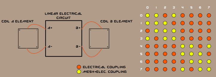
This is how I account for the electrical coupling:

Relevant project class is in https://github.com/ssrb/alternator-fem-webapp/blob/master/solver.ts

Conclusion

That was quite an entertaining project. I must now find a way to validate the results.

My references were:

• Modélisation de systèmes électrotechniques par couplage des équations électriques et magnétiques, By Fréderic Hecht, A. Marrocco, F. Piriou and A. Razek
• A general purpose method for electric and magnetic combined problems for 2D, axisymmetruc and transient systems, By P. Lombard and G.Meunier
• The Finite Element Method for Electromagnetic Modeling, By G. Meunier
• Electromagnetic Modeling by Finite Element Methods By João Pedro, A. Bastos and N. Sadowski
• Wikipedia

---

---

blog comments powered by Disqus

Published

20 January 2016

Category

Numerical methods

Tags

• mathematics 7
• electrotechnics 1