The wave penetration project: energy dissipation by bottom friction
In this post we upgrade the mild-slope equation we solved previously with a generic energy dissipation term:
where \(W( \eta )\) can account for the energy dissipated by:
- bottom friction
- wave breaking
- …
We experiment with a non-linear energy dissipation model of bottom friction implemented using simple Picard iteration. We discuss how to optimize the non-linear loop, in particular the assembly on the GPU by using graph coloring techniques.

Engage !
Energy dissipation & Bottom friction
Energy dissipation
Firstly, to better understand where this \(i \omega W( \eta )\) coefficient comes from, we need to look back at the wikipedia article and consider the time dependent mild-slope equation:
where \(\zeta: (x,y,t) \in \Omega(\mathbb{R} \times \mathbb{R}) \times \mathbb{R}^{+} \mapsto z \in \mathbb{R}\) is the real valued, time dependent free surface elevation.
This equation express an energy conservation law.
Now, if we decide that some amount of energy is lost over time, we can try to model that adding an \(-W \frac{\partial \zeta}{ \partial t}\) term to the time dependent equation.
If, again, we make the assumption that the wave motion is time harmonic, that is
we got
wich leads to the updated time harmonic version of the equation.
Note that adding the extra term to the equation changes the shape of the wave and extra care must be taken when formulating the boundary conditions. I won’t discuss it.
Bottom friction
A bottom friction energy dissipation model can be found in this old paper.
That’s quite involved and all we need to remember in the end is an expression of \(W_f(\eta)\), the energie dissipated by bottom friction:
where
\(c_f\)is a friction coeffictient;\(k\)is the wave number;\(h\)is the bathymetry
We just remark that \(W_f(\eta)\) isn’t linear with respect to \(\eta\).
Picard iteration
Picard iteration is a fixed point iteration method one can use to solve non-linear ordinary or partial differential equations.
The idea is to craft a sequence of solutions to linear PDEs which, we hope, will converge to a solution of the non-linear PDE.
We craft the linear PDEs by evaluating the non-linear coefficient with a guess which is the previous solution in the sequence.
If at some stage the solution is equal to the guess, we have converged and we know we found a solution to the non-linear PDE.
Applying that scheme to the non-linear mild-slope equation we get:
If for some \(n\) \(\eta_{n} = \eta_{n-1}\), then we found a solution to the non-linear mild-slope equation.
Here is how that scheme is implemented in C++:
const int maxNonLinearLoopIter = 42;
std::vector<std::complex<double> > eta(mesh->_vertices.size(), 0.0);
// Picard iteration, non-linear loop
for (int iter = 0; iter < maxNonLinearLoopIter; ++iter)
{
	MildSlopeEquation equation;
	Solver<std::complex<double> > solver;
	solver.solve(equation.discretize(mesh, wave, R, cf, eta), mesh, eta);
}
Optimizing
We now have a non-linear loop around the solver: it’s important to optimize what’s inside and pre-compute as much as we can out of the non-linear loop.
Since my solver is using Pardiso as a backend, it is required that blocks of the linear system are stored using the compressed row storage format (“values”, “row ptr”, “col idx”).
The profile of the CRS representation of a linear system only depends on the mesh.
The geometry and the mesh aren’t modified during Picard iteration so that we can precompute once and for all the CRS profile of the linear system, that is precompute the CRS “row ptr” and “col idx” vectors.
The “values” vector will be recomputed each iteration on the GPU.
In order to do so efficiently we also need to remember for each coefficient of the elemetary matrices its position into the “values” vector.
Here is the ocaml code doing all that:
(*
	Computes the CRS "row ptr", "col ind" as well as a mapping from elementary matrices coefficient to "values" coefficient
	ts: triangle (v1,v2,v3) list, nv: number of vertices
*)
let build_crs_profile ts nv =

	let rct = build_reverse_connectivity_table ts nv in

	(* Assembles a single row of the linear system *)
	let do_row ~init ~f row =
		rct.(row) |> List.fold ~init ~f:(fun acc ti ->
			let col0, col1, col2 = Int32.(to_int_exn ts.{ti,0}, to_int_exn ts.{ti,1}, to_int_exn ts.{ti,2}) in
			let trow = if col0 = row then 0 else if col1 = row then 1 else 2 in
			let do_col = f ti trow row
			in acc |> do_col 0 col0 |> do_col 1 col1 |> do_col 2 col2
		)
	in

	(* Simulates the assembly in order to count the number of non zero coefficients *)
	let nnz =
		(* color helps us to track already counted coeffs *)
		let color = Array.create ~len:(Array.length rct) (-1) in
		(* "fold" all the rows *)
		rct |> Array.foldi ~init:0 ~f:(fun row cnt _ ->
			row |> do_row ~init:cnt ~f:(fun ti trow row tcol col cnt ->
				(* Do not count coeffs twice *)
				if color.(col) < row then (
					color.(col) <- row;
					succ cnt
				) else
					cnt
			)
		)

	(* Perform the real assembly this time *)
	and nv = Array.length rct in

	(* color helps us to track already counted coeffs *)
	let color = Array.create ~len:nv (-1)

	(* edges helps us to remember triangles linked to an edge *)
	and edges = Array.create ~len:nnz [|(0,0); (0,0)|]

	(* The result arrays, colidx will later be converted to a BigArray as BigArray does not provide an in-place sort function *)
	and rowptr = Array1.create int32 c_layout (nv + 1)
	and colidx = Array.create ~len:nnz Int32.zero
	and tt = Array2.create int32 c_layout (Array2.dim1 ts) 9 in

	(* This sorts the nz column idx of a row before updating rowptr, colidx and tt *)
	let commit_row rstart rend =
		Array.sort ~pos:rstart ~len:(rend - rstart) ~cmp:compare colidx;
		for pos = rstart to (rend-1) do
			let col = Int32.to_int_exn colidx.(pos)
			and pos' = Int32.of_int_exn pos in
			let t0, idx0 = edges.(col).(0)
			and t1, idx1 = edges.(col).(1) in
			tt.{t0, idx0} <- pos';
			tt.{t1, idx1} <- pos'
		done
	in

	(* "fold" all the rows once again *)
 	let last = rct |> Array.foldi ~init:0 ~f:(fun row pos _ ->
		let pos' = row |> do_row ~init:pos ~f:(fun ti trow row tcol col pos ->
			let idx = 3 * trow + tcol in
			if color.(col) < row then (
				(* We found the first edge going from row to col,
					this could be the only one if it's a boundary edge *)
				color.(col) <- row;
				edges.(col).(0) <- (ti, idx);
				edges.(col).(1) <- (ti, idx);
				colidx.(pos) <- Int32.of_int_exn col;
				succ pos
			) else (
				(* there is a second edge going from row to col *)
				edges.(col).(1) <- (ti, idx);
				pos
			)
		)
		in

		(* columns idx of the current row starts at position pos and ends at position pos' - 1 *)
		rowptr.{row} <- Int32.of_int_exn pos;
		commit_row pos pos';
		pos'
	)
	in rowptr.{nv} <- Int32.of_int_exn last;

	(rowptr, (Array1.of_array int32 c_layout colidx), tt)
;;
GPU assembly revisited
The previous version of my assembler was an hybrid GPU+CPU assembler:
- elementary 3x3 matrices were computed on the GPU;
- assembling elementary matrices into a global linear system was done on the CPU
I will describe a method to perform the global assembly on the GPU too.
Data race
Here is an illustration of the data race happening when performing naive global assembly on the GPU:
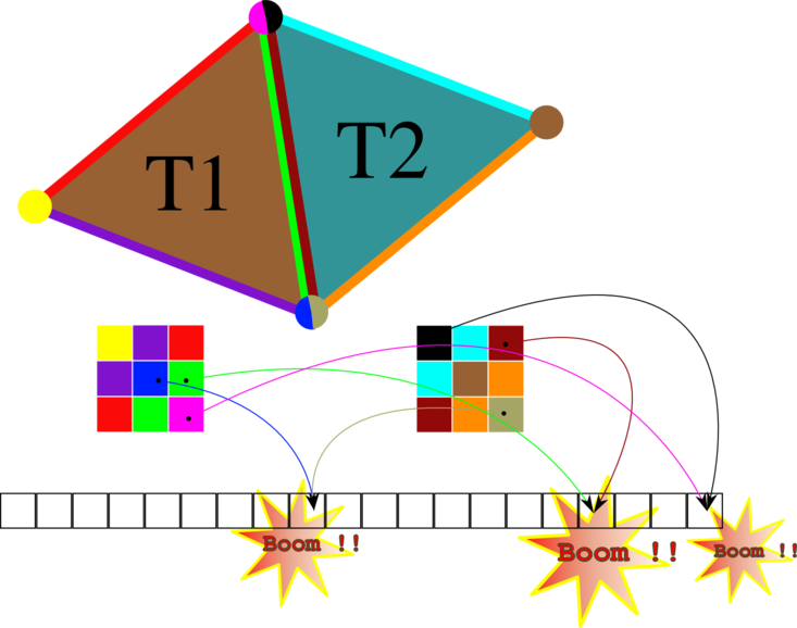
We can’t sum contributions without synchronization. On the other hand if we synchronize, we won’t get good performance.
Chordal graph and optimal coloring
In this section I will describe a method to avoid data race on the GPU based on graph coloring.
Triangle graph
In order to avoid data race between GPU threads summing contributions to a same coefficient in the global linear system, we need to make sure that not two threads are processing simultanously adjacent triangles.
Two triangles are adjacent when they share either a single vertex or a single edge (two vertices).
It’s the same as saying that not two vertices of the triangle graph (the dual graph of the mesh) are adjacent.
To build the dual graph of the mesh, first build a reverse connectivity table (a mapping from vertex to triangles)
(* ts: triangle (v1,v2,v3) list, nv: number of vertices *)
let build_reverse_connectivity_table ts nv =
	let rct = Array.create ~len:nv [] in
	List.iteri ts ~f:(fun t (v1,v2,v3) ->
		rct.(v1) <- t::rct.(v1);
		rct.(v2) <- t::rct.(v2);
		rct.(v3) <- t::rct.(v3));
	rct
;;
and then use it to efficiently connect adjacent triangles in the dual graph:
let build_triangulation_dual_graph ts nv =
	let graph = Array.create ~len:(List.length ts) [] in
	let rct = build_reverse_connectivity_table ts nv in
	List.iteri ts ~f:(fun t (v1,v2,v3) ->
		graph.(t) <- List.dedup (rct.(v1) @ rct.(v2) @ rct.(v3)));
	graph
;;
Chordal graph coloring
A chordal graph is one which every induced cycle should have at most three vertices.
By construction, the Delaunay triangulation of a convex domain is chordal.
Is the dual graph of a planar chordal graph chordal ?
I think it is (maybe suppose it’s not, and check that it implies that the primal graph wasn’t chordal in a first place ?).
A nice property of chordal graph is that it can be optimaly colored in linear time by greedy coloring vertices following a perfect elimiation order.
The perfect elimination order is computed using a lexicographic breadth-first search.
Optimaly colored means that not two adjacent triangles in the mesh will have the same color. If the GPU threads process triangles with the same color simultanously, we know that there won’t be any data race as all these triangles do not share vertices.
Here is how you color the graph using a priority queue:
let build_perfect_elemination_ordering graph =
	let compare (p1,_) (p2,_) = compare p2 p1 in
	let heap = Heap.Removable.create ~min_size:(Array.length graph) ~cmp:compare () in
	let elems = Array.mapi (fun v _ -> Heap.Removable.add_removable heap (0,v)) graph in
	let rec aux peo =
		match Heap.Removable.pop heap with
		| Some (p,v) -> List.iter graph.(v) ~f:(fun v' ->
				try
					let (p',_) = Heap.Removable.Elt.value_exn elems.(v') in
					elems.(v') <- Heap.Removable.update heap elems.(v') (succ p', v')
				with
				| _ -> ();
			);
			aux (v::peo)
		| None -> List.rev peo
	in
	aux []
;;

let do_greedy_coloring graph ordering =
	let n = Array.length graph in
	let colors = Array.create ~len:n n in
	let perfect_color v =
		let rec aux color = function
			| c::cs' -> if color < c then color else aux (succ color) cs'
			| [] -> color
		in graph.(v) |> List.map ~f:(fun v -> colors.(v)) |> List.sort ~cmp:compare |> aux 0
	in
	List.iter ordering ~f:(fun v ->
		colors.(v) <- perfect_color v
	);
	colors
;;

let graph = build_triangulation_dual_graph ts (List.length vs)
let ordering = build_perfect_elemination_ordering graph
let perfect_coloring = do_greedy_coloring graph ordering
Here is the Lyttelton test mesh colored using this algorithm. It uses 9 colors.
Improving the GPU assembly
Updating the GPU code to take advantage of the coloring is easy enough. All we need to do now is call the assembly kernel as many times as there are colors.
A GPU thread will only sum contributions of its triangle if it has the requested color:
Host code:
// Coloring computed by the greedy coloring algorithm
device_vector<int> colorsOnGpu(colors, &colors[nt]);

// tt is the mapping from local triangle element coefficient index
// to the index in the global linear system compressed row storage values
device_vector<int> ttOnGpu(tt, &tt[9 * nt]);

// Compressed row storage values on the GPU, initialized to 0 before summing
device_vector<float> result(rowptr[nv]);
fill(result.begin(), result.end(), 0.);

// How many colors ?
device_vector<int>::iterator maxIter = max_element(colorsOnGpu.begin(), colorsOnGpu.end());
int nbColor = 1 + *maxIter;
for (int color = 0; color < nbColor; ++color)
{
	// Only assemble triangles with that color
	Assemble<<<nbBlock, trianglesPerBlock>>>(
	  coeffsOnGpu,
	  colorsOnGpu,
	  ttOnGpu,
	  result,
	  color
	);
}
copy(coeffsOnGpu.begin(), coeffsOnGpu.end(), coeffs);
Device code:
__global__
  void Assemble(
    const KernelArray<float> coeffs,
    const KernelArray<color_t> colors,
    const KernelArray<int> tt,
    KernelArray<float> result,
    color_t color) {
    const int myTriangleId = blockIdx.x * blockDim.x + threadIdx.x;
    if (myTriangleId < colors.size() && colors[myTriangleId] == color) {
      const int *mytt = &tt[9 * myTriangleId];
      const float *myCoeffs = &coeffs[9 * myTriangleId];
      result[mytt[0]] += myCoeffs[0];
      result[mytt[1]] += myCoeffs[1];
      result[mytt[2]] += myCoeffs[2];
      result[mytt[3]] += myCoeffs[3];
      result[mytt[4]] += myCoeffs[4];
      result[mytt[5]] += myCoeffs[5];
      result[mytt[6]] += myCoeffs[6];
      result[mytt[7]] += myCoeffs[7];
      result[mytt[8]] += myCoeffs[8];
    }
  }
Conclusion
- My
C++solver for the non-linear mild-slope equation can be found on my github; - The
ocaml/CUDAassembler based on graph coloring can be found on my github
This method is easy enough to implement and can be applied to other type of accelerator such as the Xeon Phi.
There exist other parallel FEM assembly alogrithms targetting massively parallel architectures that I will try to implement.
My main references were:
- Assembly of Finite Element Methods on Graphics Processors, By Cris Cecka, Adrian J. Lew and E. Darve
- An efficient way to perform the assembly of finite element matrices in Matlab and Octave, By François Cuvelier, Caroline Japhet and Gilles Scarella
- Simple linear-time algorithms to test chordality of graphs, test acyclicity of hypergraphs and selectively reduce acyclic hypergraphs by Robert E. Tarjan and Mihalis Yannakakis
- Wikipedia
blog comments powered by Disqus